Chapter 1 Linear Programming Paragraph 5 Duality What we did so - PowerPoint PPT Presentation
Chapter 1 Linear Programming Paragraph 5 Duality What we did so far We developed the 2-Phase Simplex Algorithm: Hop (reasonably) from basic solution (bs) to bs until you find a basic feasible solution (bfs) or until it becomes clear
Chapter 1 Linear Programming Paragraph 5 Duality
What we did so far • We developed the 2-Phase Simplex Algorithm: – Hop (reasonably) from basic solution (bs) to bs until you find a basic feasible solution (bfs) or until it becomes clear that none exists. – Hop from bfs to bfs until you cannot find an improving solution or the improving trajectory is unbounded. • We have seen that we can guarantee termination but that the worst-case runtime is exponential. • Again: Note that LP is polynomial time solvable! CS 149 - Intro to CO 2
Lower Bounds on the Objective • Let π ∈ Ñ m , π ≥ 0. Consider two sets: – P 1 = {x ∈ Ñ n | Ax ≥ b, x ≥ 0} and – P 2 = {x ∈ Ñ n | π T Ax ≥ π T b, x ≥ 0}. • Since π ≥ 0, it is clear that P 1 Œ P 2 , in other words: For all x ∈ P 1 we have that π T Ax ≥ π T b. • Now assume that π ≥ 0 and also π T A ≤ c T . Then, for all x ∈ P 1 , we have that π T b ≤ π T Ax ≤ c T x. • Therefore, every such π provides us with a lower bound on the objective! CS 149 - Intro to CO 3
Duality • The problem of finding the best such lower bound π T b with π ∈ Ñ such that π T A ≤ c T , π ≥ 0 is called the Dual Problem of (P 1 ,c). • Formally, let P 3 = { π ∈ Ñ m | A T π ≤ c, π ≥ 0}. Then, (P 3 ,b) is called the dual of the primal (P 1 ,c). • Theorem – The dual of the dual is the primal. – For all primal feasible x and dual feasible π it holds that π T b ≤ c T x [weak duality]. CS 149 - Intro to CO 4
Example • Minimize x 1 +3x 2 +x 3 such that – 2x 1 +x 2 ≥ 3 – -x 1 +x 3 ≥ 4 (P) – x 1 , x 2 , x 3 ≥ 0 π 1 is dual feasible • π 1T = (1/2,1) ⇒ Relax P 1 to and shows: every feasible x (if any • 0.5x 2 +x 3 ≥ 5.5 exists!) has an • x 1 , x 2 , x 3 ≥ 0 objective value of • Maximize 3 π 1 +4 π 2 such that at least 5.5! – 2 π 1 - π 2 ≤ 1 – 0 ≤ π 1 ≤ 3 (D) – 0 ≤ π 2 ≤ 1 CS 149 - Intro to CO 5
Example • Minimize x 1 +3x 2 +x 3 such that – 2x 1 +x 2 ≥ 3 – -x 1 +x 3 ≥ 4 (P) – x 1 , x 2 , x 3 ≥ 0 π 0 is dual optimal • π 0T = (1,1) ⇒ Relax P 1 to and shows: every feasible x (if any • x1+x2+x3 ≥ 7 exists!) has an • x 1 , x 2 , x 3 ≥ 0 objective value of • Maximize 3 π 1 +4 π 2 such that at least 7! – 2 π 1 - π 2 ≤ 1 – 0 ≤ π 1 ≤ 3 (D) – 0 ≤ π 2 ≤ 1 CS 149 - Intro to CO 6
The Dual of the Standard Form • P 1 = {x ∈ Ñ n | Ax = b, x ≥ 0} (LP) S = (P 1 ,c) • P 2 = {x ∈ Ñ n | Ax ≥ b, -Ax ≥ -b, x ≥ 0} (LP) C = (P 2 ,c) • P 3 = {( η , μ ) ∈ Ñ m | A T η - A T μ ≤ c, η , μ ≥ 0} @ P 4 = { π ∈ Ñ m | A T π ≤ c} [ π not non-negative anymore!] • The dual of (LP) S is therefore (P 4 ,b). CS 149 - Intro to CO 7
The Dual of Unspecified Forms • Max b T π • Min c T x – π M+ ≥ 0 – A M+ x ≥ b + – π M0 unrestricted – A M0 x = b � – π M- ≤ 0 – A M- x ≤ b - – (A T ) N+ π – x N+ ≥ 0 ≤ c N+ – (A T ) N0 π = c N0 – x N0 unrestricted – (A T ) N- π – x N- ≤ 0 ≥ c N- M+ ∪ M0 ∪ M- = {1,..,m} N+ ∪ N0 ∪ N- = {1,..,n} CS 149 - Intro to CO 8
Strong Duality c T = c T – c B T A B -1 A -c T x 0 A B -1 A A B -1 b • Given is an LP in standard form. • We know: The current bfs x 0 in the tableau is optimal when c T – c BT A B-1 A ≥ 0 ñ (c BT A B-1 ) A ≤ c. • Therefore, π T := c BT A B-1 is dual feasible! • But: π T b = c BT A B-1 b = c BT x B0 = c T x 0 ! ☺ CS 149 - Intro to CO 9
Duality • The problem of finding the best such lower bound π T b with π ∈ Ñ such that π T A ≤ c T , π ≥ 0 is called the Dual Problem of (P 1 ,c). • Formally, let P 3 = { π ∈ Ñ m | A T π ≤ c, π ≥ 0}. Then, (P 3 ,b) is called the dual of the primal (P 1 ,c). • Theorem – The dual of the dual is the primal. – For all primal feasible x and dual feasible π it holds that π T b ≤ c T x [weak duality]. – For primal optimal x 0 and dual optimal π 0 it holds that π 0T b = c 0T x [strong duality]. CS 149 - Intro to CO 10
Complementary Slackness • Consider an LP in canonical form with x 0 primal optimal, and π 0 dual optimal. • c T x 0 = π 0T b ≤ π 0T Ax 0 ≤ c T x 0 ⇒ π 0T (Ax 0 -b) = 0. • π 0T b = c T x 0 ≥ π 0T Ax 0 ≥ π 0T b ⇒ (c T - π 0T A) x 0 = 0. • Consequently, since π 0 , Ax 0 -b ≥ 0, π 0 can only have non-zero components where there is no slack in the corresponding primal constraint. • Analogously, since x 0 , c T - π 0T A ≥ 0, x 0 can only have non-zero components where there is no slack in the corresponding dual constraint. CS 149 - Intro to CO 11
Relation of Primal and Dual Dual Finite Unbounded Infeasible Optimum Primal Finite � [sd] � [wd] � [sd] Optimum � [wd] � [wd] � [wd] Unbounded � [sd] � [wd] � Infeasible wd – weak duality sd – strong duality CS 149 - Intro to CO 12
Farkas’ Lemma • Given are a i ∈ Ñ n ,1 ≤ i ≤ m, and a vector c ∈ Ñ n . • The cone of the a i is defined as the set C(a 1 ,..,a m ) := {x ∈ Ñ n | x = Σ π i a i , π i ≥ 0}. • Farkas’ Lemma – (For all y with y T a i ≥ 0 for all i it holds y T c ≥ 0) ⇔ – c ∈ C(a 1 ,..,a m ). • Proof: Exercise! CS 149 - Intro to CO 13
The Dual Simplex Algorithm • We have seen how we compute a dual optimal solution after having solved the primal with the simplex algorithm. • Consequently, we can solve the primal by solving the dual! • In case that c ≥ 0, π = 0 is dual feasible – so we may save the effort for solving phase I when focusing on the dual right away. • Example: Transportation Problem, Diet Problem, Shortest Path, … CS 149 - Intro to CO 14
The Dual Simplex Algorithm • Recall that the dual works by looking at –A T instead of A in the tableau. • Consequently, we can simply exchange the roles of rows and columns and consider matrix entries with opposite sign. • Assume we are dual feasible. Then: – Search for a row with negative b i . (no such i ⇒ dual optimal ⇒ primal feasible) – Find a column j such that a ij < 0 and c j / -a ij is minimal! (no such j ⇒ dual unbounded ⇒ primal infeasible) – Pivot around a ij . CS 149 - Intro to CO 15
The Dual Simplex Algorithm • Consider our instance of the diet problem: CS 149 - Intro to CO 16
Examples – Diet Problem B M Amount needed [g] Cost/kg 20 15 Minimize 25M + 15B [$] Carbs 10 25 500 10M + 25B ¥ 50 [%] Fat [%] 10 5 250 10M + 5B ¥ 25 Protein 15 20 600 15M + 20B ¥ 60 [%] CS 149 - Intro to CO 17
The Dual Simplex Algorithm • Consider our instance of the diet problem: B 0 0 0 25 15 0 5 $ 4 1 0 0 -10 -25 -50 2 0 1 0 -10 -5 -25 0 0 0 1 -15 -20 -60 M 0 2 4 5 CS 149 - Intro to CO 18
The Dual Simplex Algorithm • Consider our instance of the diet problem: B 0 0 3/4 55/4 0 -45 5 $ 4 1 0 -5/4 35/4 0 25 2 0 1 -1/4 -25/4 0 -10 0 0 -1/20 3/4 1 3 M 0 2 4 5 CS 149 - Intro to CO 19
The Dual Simplex Algorithm • Consider our instance of the diet problem: B 0 11/5 1/5 0 0 -67 5 $ 4 1 7/5 -8/5 0 0 11 2 0 -4/25 1/25 1 0 8/5 0 0 3/25 -4/25 0 1 9/5 M 0 2 4 5 CS 149 - Intro to CO 20
Shadow Prices • Consider production planning. In the optimal tableau, the relative costs of the slack variables are exactly -c B T A B -1 . • Note that the objective in the simplex was to minimize. Thus, the relative costs of slack variables give us the dual solution. • If a slack variable is not in the basis, it is 0 in the optimal solution. I.e. the corresponding constraint is tight for optimality. • Now, the relative costs tell us, how much we could gain if the constraint was not tight. Consequently, the optimal duals are called “shadow prices” of their corresponding constraints. CS 149 - Intro to CO 21
Thank you! Thank you!
Recommend
More recommend
Explore More Topics
Stay informed with curated content and fresh updates.
