Duality Geoff Gordon & Ryan Tibshirani Optimization 10-725 / - PowerPoint PPT Presentation
Duality Geoff Gordon & Ryan Tibshirani Optimization 10-725 / 36-725 1 Duality in linear programs Suppose we want to find lower bound on the optimal value in our convex problem, B min x C f ( x ) E.g., consider the following simple
Duality Geoff Gordon & Ryan Tibshirani Optimization 10-725 / 36-725 1
Duality in linear programs Suppose we want to find lower bound on the optimal value in our convex problem, B ≤ min x ∈ C f ( x ) E.g., consider the following simple LP min x + y x,y subject to x + y ≥ 2 x, y ≥ 0 What’s a lower bound? Easy, take B = 2 But didn’t we get “lucky”? 2
Try again: min x + 3 y x + y ≥ 2 x,y + 2 y ≥ 0 subject to x + y ≥ 2 = x + 3 y ≥ 2 x, y ≥ 0 Lower bound B = 2 More generally: min px + qy a + b = p x,y a + c = q subject to x + y ≥ 2 a, b, c ≥ 0 x, y ≥ 0 Lower bound B = 2 a , for any a, b, c satisfying above 3
What’s the best we can do? Maximize our lower bound over all possible a, b, c : min px + qy max a,b,c 2 a x,y subject to x + y ≥ 2 subject to a + b = p x, y ≥ 0 a + c = q a, b, c ≥ 0 Called primal LP Called dual LP Note: number of dual variables is number of primal constraints 4
Try another one: min px + qy max a,b,c 2 c − b x,y subject to x ≥ 0 subject to a + 3 c = p y ≤ 1 − b + c = q 3 x + y = 2 a, b ≥ 0 Primal LP Dual LP Note: in the dual problem, c is unconstrained 5
General form LP Given c ∈ R n , A ∈ R m × n , b ∈ R m , G ∈ R r × n , h ∈ R r x ∈ R n c T x u ∈ R m ,v ∈ R r − b T u − h T v min max subject to − A T u − G T v = c subject to Ax = b Gx ≤ h v ≥ 0 Primal LP Dual LP Explanation: for any u and v ≥ 0 , and x primal feasible, u T ( Ax − b ) + v T ( Gx − h ) ≤ 0 , i.e., ( − A T u − G T v ) T x ≥ − b T u − h T v So if c = − A T u − G T v , we get a bound on primal optimal value 6
Max flow and min cut Soviet railway network (from Schrijver (2002), On the history of transportation and maximum flow problems ) 7
s Given graph G = ( V, E ) , define flow f ij , ( i, j ) ∈ E to satisfy: • f ij ≥ 0 , ( i, j ) ∈ E f ij • f ij ≤ c ij , ( i, j ) ∈ E c ij � � • f ik = f kj , k ∈ V \{ s, t } ( i,k ) ∈ E ( k,j ) ∈ E t Max flow problem: find flow that maximizes total value of flow from s to t . I.e., as an LP: � max f sj f ∈ R | E | ( s,j ) ∈ E subject to f ij ≥ 0 , f ij ≤ c ij for all ( i, j ) ∈ E � � f ik = f kj for all k ∈ V \ { s, t } ( i,k ) ∈ E ( k,j ) ∈ E 8
Derive the dual, in steps: • Note that � � � − a ij f ij + b ij ( f ij − c ij ) ( i,j ) ∈ E � � � � � + x k f ik − f kj ≤ 0 k ∈ V \{ s,t } ( i,k ) ∈ E ( k,j ) ∈ E for any a ij , b ij ≥ 0 , ( i, j ) ∈ E , and x k , k ∈ V \ { s, t } • Rearrange as � � M ij ( a, b, x ) f ij ≤ b ij c ij ( i,j ) ∈ E ( i,j ) ∈ E where M ij ( a, b, x ) collects terms multiplying f ij 9
• Want to make LHS in previous inequality equal to primal M sj = b sj − a sj + x j want this = 1 objective, i.e., M it = b it − a it − x i want this = 0 M ij = b ij − a ij + x j − x i want this = 0 • We’ve shown that � primal optimal value ≤ b ij c ij , ( i,j ) ∈ E subject to a, b, x satisfying constraints. Hence dual problem is (minimize over a, b, x to get best upper bound): � min b ij c ij b ∈ R | E | ,x ∈ R | V | ( i,j ) ∈ E subject to b ij + x j − x i ≥ 0 for all ( i, j ) ∈ E b ≥ 0 , x s = 1 , x t = 0 10
Suppose that at the solution, it just so happened x i ∈ { 0 , 1 } for all i ∈ V Call A = { i : x i = 1 } and B = { i : x i = 0 } , note that s ∈ A and t ∈ B . Then the constraints b ij ≥ x i − x j for ( i, j ) ∈ E, b ≥ 0 imply that b ij = 1 if i ∈ A and j ∈ B , and 0 otherwise. Moreover, the objective � ( i,j ) ∈ E b ij c ij is the capacity of cut defined by A, B I.e., we’ve argued that the dual is the LP relaxation of the min cut problem: � min b ij c ij b ∈ R | E | ,x ∈ R | V | ( i,j ) ∈ E subject to b ij ≥ x i − x j b ij , x i , x j ∈ { 0 , 1 } for all i, j 11
Therefore, from what we know so far: value of max flow ≤ optimal value for LP relaxed min cut ≤ capacity of min cut Famous result, called max flow min cut theorem: value of max flow through a network is exactly the capacity of the min cut Hence in the above, we get all equalities. In particular, we get that the primal LP and dual LP have exactly the same optimal values, a phenomenon called strong duality How often does this happen? More on this later 12
(From F. Estrada et al. (2004), “Spectral embedding and min cut for image segmentation”) 13
Another perspective on LP duality x ∈ R n c T x u ∈ R m , v ∈ R r − b T u − h T v min max subject to − A T u − G T v = c subject to Ax = b Gx ≤ h v ≥ 0 Primal LP Dual LP Explanation # 2: for any u and v ≥ 0 , and x primal feasible c T x ≥ c T x + u T ( Ax − b ) + v T ( Gx − h ) := L ( x, u, v ) So if C denotes primal feasible set, f ⋆ primal optimal value, then for any u and v ≥ 0 , f ⋆ ≥ min x ∈ C L ( x, u, v ) ≥ min x ∈ R n L ( x, u, v ) := g ( u, v ) 14
In other words, g ( u, v ) is a lower bound on f ⋆ for any u and v ≥ 0 Note that � − b T u − h T v if c = − A T u − G T v g ( u, v ) = −∞ otherwise Now we can maximize g ( u, v ) over u and v ≥ 0 to get the tightest bound, and this gives exactly the dual LP as before This last perspective is actually completely general and applies to arbitrary optimization problems (even nonconvex ones) 15
Outline Rest of today: • Lagrange dual function • Langrange dual problem • Examples • Weak and strong duality 16
Lagrangian Consider general minimization problem x ∈ R n f ( x ) min subject to h i ( x ) ≤ 0 , i = 1 , . . . m ℓ j ( x ) = 0 , j = 1 , . . . r Need not be convex, but of course we will pay special attention to convex case We define the Lagrangian as m r � � L ( x, u, v ) = f ( x ) + u i h i ( x ) + v j ℓ j ( x ) i =1 j =1 New variables u ∈ R m , v ∈ R r , with u ≥ 0 (implicitly, we define L ( x, u, v ) = −∞ for u < 0 ) 17
Important property: for any u ≥ 0 and v , f ( x ) ≥ L ( x, u, v ) at each feasible x Why? For feasible x , m r � � L ( x, u, v ) = f ( x ) + u i h i ( x ) + v j ℓ j ( x ) ≤ f ( x ) � �� � � �� � i =1 j =1 ≤ 0 =0 • Solid line is f • Dashed line is h , hence feasible set ≈ [ − 0 . 46 , 0 . 46] • Each dotted line shows L ( x, u, v ) for different choices of u ≥ 0 and v (From B & V page 217) 18
Lagrange dual function Let C denote primal feasible set, f ⋆ denote primal optimal value. Minimizing L ( x, u, v ) over all x ∈ R n gives a lower bound: f ⋆ ≥ min x ∈ C L ( x, u, v ) ≥ min x ∈ R n L ( x, u, v ) := g ( u, v ) We call g ( u, v ) the Lagrange dual function , and it gives a lower bound on f ⋆ for any u ≥ 0 and v , called dual feasible u, v • Dashed horizontal line is f ⋆ • Dual variable λ is (our u ) • Solid line shows g ( λ ) (From B & V page 217) 19
Quadratic program Consider quadratic program (QP, step up from LP!) 1 2 x T Qx + c T x min x ∈ R n subject to Ax = b, x ≥ 0 where Q ≻ 0 . Lagrangian: L ( x, u, v ) = 1 2 x T Qx + c T x − u T x + v T ( Ax − b ) Lagrange dual function: x ∈ R n L ( x, u, v ) = − 1 2( c − u + A T v ) T Q − 1 ( c − u + A T v ) − b T v g ( u, v ) = min For any u ≥ 0 and any v , this is lower a bound on primal optimal value f ⋆ 20
Same problem 1 2 x T Qx + c T x min x ∈ R n subject to Ax = b, x ≥ 0 but now Q � 0 . Lagrangian: L ( x, u, v ) = 1 2 x T Qx + c T x − u T x + v T ( Ax − b ) Lagrange dual function: 2 ( c − u + A T v ) T Q + ( c − u + A T v ) − b T v − 1 if c − u + A T v ⊥ null( Q ) g ( u, v ) = −∞ −∞ otherwise where Q + denotes generalized inverse of Q . For any u ≥ 0 , v , and c − u + A T v ⊥ null( Q ) , g ( u, v ) is a nontrivial lower bound on f ⋆ 21
Quadratic program in 2D We choose f ( x ) to be quadratic in 2 variables, subject to x ≥ 0 . Dual function g ( u ) is also quadratic in 2 variables, also subject to u ≥ 0 Dual function g ( u ) provides a bound on f ⋆ for every u ≥ 0 primal f / g Largest bound this ● ● gives us: turns out to be exactly f ⋆ ... dual coincidence? More on this later x1 / u1 x2 / u2 22
Lagrange dual problem Given primal problem x ∈ R n f ( x ) min subject to h i ( x ) ≤ 0 , i = 1 , . . . m ℓ j ( x ) = 0 , j = 1 , . . . r Our constructed dual function g ( u, v ) satisfies f ⋆ ≥ g ( u, v ) for all u ≥ 0 and v . Hence best lower bound is given by maximizing g ( u, v ) over all dual feasible u, v , yielding Lagrange dual problem: u ∈ R m , v ∈ R r g ( u, v ) max subject to u ≥ 0 Key property, called weak duality: if dual optimal value g ⋆ , then f ⋆ ≥ g ⋆ Note that this always holds (even if primal problem is nonconvex) 23
Another key property: the dual problem is a convex optimization problem (as written, it is a concave maximization problem) Again, this is always true (even when primal problem is not convex) By definition: m r � � � � g ( u, v ) = min f ( x ) + u i h i ( x ) + v j ℓ j ( x ) x ∈ R n i =1 j =1 m r � � � � = − max − f ( x ) − u i h i ( x ) − v j ℓ j ( x ) x ∈ R n i =1 j =1 � �� � pointwise maximum of convex functions in ( u, v ) I.e., g is concave in ( u, v ) , and u ≥ 0 is a convex constraint, hence dual problem is a concave maximization problem 24
Recommend
More recommend
Explore More Topics
Stay informed with curated content and fresh updates.
