III. 9. IS LM: the basic framework to understand macro policy Text, - PDF document
III. 9. IS LM: the basic framework to understand macro policy Text, ch 10 49 Objectives: To understand the factors which determine the level of output in the short-run. To learn how, in the short run, the level of interest rates [ r ]
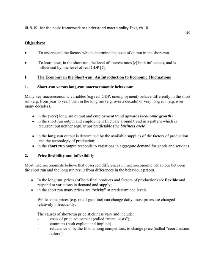
III. 9. IS ‐ LM: the basic framework to understand macro policy Text, ch 10 49 Objectives: To understand the factors which determine the level of output in the short-run. To learn how, in the short run, the level of interest rates [ r ] both influences, and is influenced by, the level of real GDP [ Y ]. I. The Economy in the Short-run: An Introduction to Economic Fluctuations 1. Short-run versus long-run macroeconomic behaviour Many key macroeconomic variables (e.g real GDP, unemployment) behave differently in the short run (e.g. from year to year) than in the long run (e.g. over a decade) or very long run (e.g. over many decades). in the (very) long run output and employment trend upwards ( economic growth ) in the short run output and employment fluctuate around trend in a pattern which is recurrent but neither regular nor predictable (the business cycle ). in the long run output is determined by the available supplies of the factors of production and the technology of production; in the short run output responds to variations in aggregate demand for goods and services. 2. Price flexibility and inflexibility Most macroeconomists believe that observed differences in macroeconomic behaviour between the short run and the long run result from differences in the behaviour prices. In the long run, prices (of both final products and factors of production) are flexible and respond to variations in demand and supply; in the short run many prices are “sticky” at predetermined levels. While some prices (e.g. retail gasoline) can change daily, most prices are changed relatively infrequently. The causes of short-run price stickiness vary and include: - costs of price adjustment (called “menu costs”); - contracts (both explicit and implicit) - reluctance to be the first, among competitors, to change price (called “coordination failure”).
III. 9. IS ‐ LM: the basic framework to understand macro policy Text, ch 10 50 3. A short-run aggregate demand and supply model In chapters 10 and 11, we utilize a (Keynesian) model of short run output determination based on two key assumptions about aggregate supply: all prices are stuck at predetermined levels in the short run and, hence, there is a given, predetermined value of the aggregate price level , denoted as P ; firms are willing to produce and sell as much output as buyers are willing to buy at given prices. The Keynesian-Cross Model of Output Determination. II. the simplest interpretation of Keynes’s theory of short-run output determination; ignores the impact of interest rates and monetary policy; is a building block for the more complex and realistic IS-LM model. The determinants of planned expenditure [PE ] in the Keynesian-Cross model. 1. Assume a closed economy: NX =0 and so: PE = C + I + G Consumption [ C ] is an increasing function of aggregate disposable income [ Y-T ]: C = C(Y - T) 0 < MPC < 1, MPC= Δ C / Δ ( Y-T ) Planned investment spending is assumed to be an exogenous variable whose value is determined outside the model: I I Both govt. spending on output and taxes are assumed to be exogenous , determined outside the model by fiscal policy: G G T T
III. 9. IS ‐ LM: the basic framework to understand macro policy Text, ch 10 51 The planned expenditure function. 2. PE = C + I + G P E C ( Y T ) I G Planned aggregate expenditure is a function of: real GDP [ Y ]; exogenous level of planned investment spending [ I ]; and exogenous fiscal policy variables [ G and T ]. The planned expenditure curve . 3. It shows how PE varies with Y when I , G , and T are held constant. PE increases with Y because C increases with Y : Y ↑ → ( Y - T ) ↑ → C ↑ → PE ↑ The slope of the PE curve equals the MPC: E E Slope MPC ( Y T ) ( Y T ) The equilibrium of the economy. 4. Definition: The level of Y such that Y = PE is called the equilibrium level of output, Y e The process of adjustment to equilibrium. Suppose, initially, Y = Y 1 > Y e When Y = Y 1 , PE = PE 1 < Y 1 . Firms are selling less than they are producing. Unsold output results in unplanned inventory accumulation. unplanned inventory increase → firms reduce production → Y falls Adjustment mechanism: unplanned inventory decreas → firms increase production → Y ↑
III. 9. IS ‐ LM: the basic framework to understand macro policy Text, ch 10 52 So: firms react to this unplanned inventory build-up by reducing production levels to match demand: Y falls until Y = PE. Output falls until actual expenditure = planned expenditure Why is Y equal to actual expenditure? Because actual expenditure includes both planned and unplanned changes in inventories. In a closed economy, whatever is produced can be: Bought by consumers Bought by government Bought for investment purposes (this is planned investment) and whatever is left over ends up in inventory Note: as Y falls, PE falls as well. But Y falls faster: PE falls by the decrease in Y times the marginal propensity to consume: ∆ PE=MPC· ∆ (Y- T ) At home: analyse what happens when Y = Y 1 < Y e Analysis of various changes. 6. We will always start initially in equilibrium at point A where: Y = Y e = PE An increase in G . A) PE ↑ PE > Y 1 G ↑ unplanned inventory drop firms react by producing more Y ↑ C ↑ [ ∆ C = MPC· ∆ (Y- T )] PE ↑ [ ∆ E = ∆ C +I+G] both Y ↑ and E ↑ but Y rises faster until Y = Y 2 = PE 2
III. 9. IS ‐ LM: the basic framework to understand macro policy Text, ch 10 53 The government purchases multiplier : Initial increase in G raises output by the same amount; as Y ↑ consumption rises as well, increasing Y further; So: final increase in Y exceeds the initial increase in G . Def: The govt. purchases multiplier is the amount by which equilibrium Y changes, following a one-unit increase in G : Y Govt. purchases multiplier G Deriving the multiplier . Y C ( Y T ) I G e e After an increase in G : ∆ Y e = MPC ∆ Y e + ∆ G ∆ Y e (1- MPC ) = ∆ G G ∆ Y e = ( 1 MPC ) Y e 1 G ( 1 MPC ) The larger [smaller] is the MPC the larger [smaller] is the multiplier of equilibrium income with respect to a change in govt. spending. A decrease in taxes. B) A drop in taxes raises consumption at each level of Y by - MPC· ∆ T A tax cut of $1.00 has the same effect on Y e as an increase in G equal to MPC ·$1
III. 9. IS ‐ LM: the basic framework to understand macro policy Text, ch 10 54 The tax multiplier formula: We have: Y C ( Y T ) I G e e After an increase in T : ∆ Y e = MPC ∆ Y e - MPC ∆ T ∆ Y e (1- MPC) = - MPC ∆ T ∆ Y e = - MPC ∆ T (1-MPC) Y e MPC T ( 1 MPC ) The multiplier in practice . MPC for Canada = 0.75. So, by our simple formula: 1/(1-MPC)=4. But in fact the multiplier is considerably lower than that due to two factors which are ignored by our simple formula: (a) As income increases, disposable income increases less because income taxes increase and subsidies fall Y ↑ by $1 → T ↑ by $0.4 (taxes increase by $0.25, subsidies fall by $0.15) We can write it as: T=T 0 + 0.4 Y . So: PE C Y [ ( T 0.4 )] Y I G o So: if Y ↑ by $1 → disposable income ( Y-T ) ↑ by 60 cents only (b) Part of the extra spending is on imports : 75 cents of each $1 ↑ in disposable income is spent, but only 75% of that increased spending is on Canadian-produced output, with 25% on imports. We can write it as:
III. 9. IS ‐ LM: the basic framework to understand macro policy Text, ch 10 55 NX= EX-IM 0 -0. 25[ Y- ( T 0 + 0.4 Y )] Inserting into the equation for PE: PE C Y [ ( T 0.4 )] Y I G NX o PE C Y [ ( T 0.4 )] Y I G EX IM 0.25 Y T 0.4 Y o 0 0 PE 0.75 [ C Y ( T 0.4 )] Y I G EX IM o 0 So the effect of an increase in Y by $1 on aggregate expenditure is, since the MPC is 0.75: 0.75 x 0.6 x 0.75 = 0.34 Imposing in equilibrium PE= Y e . So if G changes: ∆ Y e = 0.75 MPC ∆ Y e (1-0.4) + ∆ G = 0.34 ∆ Y e + ∆ G So the multiplier is 1/(1-0.34) = 1.5 Below we will abstract from the effect of income on taxes and on imports. The IS Curve. III. We will now develop the IS-LM model . The Keynesian- cross is the basis for IS curve which shows the equilibrium in the goods market. To obtain - replace the assumption of exogenous investment with the investment function. The investment function. 1. I = I ( r ), where: r ↑ → I ↓
Recommend
More recommend
Explore More Topics
Stay informed with curated content and fresh updates.
