Trust region policy optimization (TRPO) Value Iteration Value - PowerPoint PPT Presentation
Trust region policy optimization (TRPO) Value Iteration Value Iteration This is what we similar to what Q-Learning does, the main difference being that we we might not know the actual expected reward and instead explore the world and use
Trust region policy optimization (TRPO)
Value Iteration
Value Iteration • This is what we similar to what Q-Learning does, the main difference being that we we might not know the actual expected reward and instead explore the world and use discounted rewards to model our value function.
Model-based Value Iteration Model-free • This is what we similar to what Q-Learning does, the main difference being that we we might not know the actual expected reward and instead explore the world and use discounted rewards to model our value function.
Value Iteration • This is what we similar to what Q-Learning does, the main difference being that we we might not know the actual expected reward and instead explore the world and use discounted rewards to model our value function. • Once we have Q(s,a), we can find optimal policy π * using:
Policy Iteration • We can directly optimize in the policy space.
Policy Iteration Smaller than Q-function space • We can directly optimize in the policy space.
Preliminaries Following identity expresses the expected return of another policy in terms of the advantage over π, accumulated over time steps: Where A π is the advantage function: And is the visitation frequency of states in policy
Preliminaries To remove the complexity due to , following local approximation is introduced: If we have a parameterized policy , where is a differentiable function of the parameter vector , then matches to first order. i.e., This implies that a sufficiently small step that improves will also improve , but does not give us any guidance on how big of a step to take.
Preliminaries • To address this issue, Kakade & Langford (2002) proposed conservative policy iteration: where, • They derived the following lower bound:
Preliminaries • Computationally, this α-coupling means that if we randomly choose a seed for our random number generator, and then we sample from each of π and π new after setting that seed, the results will agree for at least fraction 1-α of seeds. • Thus α can be considered as a measure of disagreement between π and π new
Theorem 1 • Previous result was applicable to mixture policies only. Schulman showed that it can be extended to general stochastic policies by using a distance measure called “Total Variation” divergence between π and as : for discrete probability distributions p; q • Let • They proved that for , following result holds:
Theorem 1 • Note the following relation between Total Variation & Kullback–Leibler: • Thus bounding condition becomes:
Algorithm 1
Trust Region Policy Optimization • For parameterized policies with parameter vector, we are guaranteed to improve the true objective by performing following maximization: • However, using the penalty coefficient like above results in very small step sizes. One way to take larger steps in a robust way is to use a constraint on the KL divergence between the new policy and the old policy, i.e., a trust region constraint :
Trust Region Policy Optimization • The constraint is bounded at every point in state space, which is not practical. We can use the following heuristic approximation: • Thus, the optimization problem becomes:
Trust Region Policy Optimization • In terms of expectation, previous equation can be written as: where, q denotes the sampling distribution • This sampling distribution can be calculated in two ways: Ø a) Single Path Method Ø b) Vine Method
Final Algorithm • Step 1: Use the single path or vine procedures to collect a set of state-action pairs along with Monte Carlo estimates of their Q -values • Step 2: By averaging over samples, construct the estimated objective and constraint in Equation (14) • Step 3: Approximately solve this constrained optimization problem to update the policy’s parameter vector
Recommend
More recommend
Explore More Topics
Stay informed with curated content and fresh updates.
