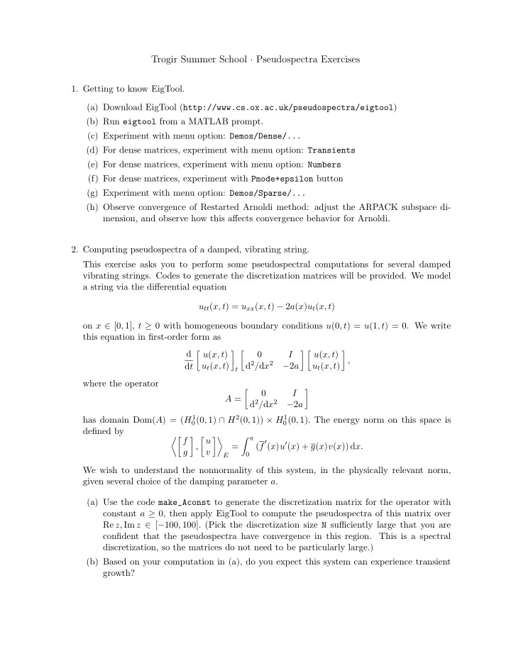
Trogir Summer School Pseudospectra Exercises 1. Getting to know - PDF document

Trogir Summer School · Pseudospectra Exercises 1. Getting to know EigTool. (a) Download EigTool ( http://www.cs.ox.ac.uk/pseudospectra/eigtool ) (b) Run eigtool from a MATLAB prompt. (c) Experiment with menu option: Demos/Dense/... (d) For dense matrices, experiment with menu option: Transients (e) For dense matrices, experiment with menu option: Numbers (f) For dense matrices, experiment with Pmode+epsilon button (g) Experiment with menu option: Demos/Sparse/... (h) Observe convergence of Restarted Arnoldi method: adjust the ARPACK subspace di- mension, and observe how this affects convergence behavior for Arnoldi. 2. Computing pseudospectra of a damped, vibrating string. This exercise asks you to perform some pseudospectral computations for several damped vibrating strings. Codes to generate the discretization matrices will be provided. We model a string via the differential equation u tt ( x, t ) = u xx ( x, t ) − 2 a ( x ) u t ( x, t ) on x ∈ [0 , 1], t ≥ 0 with homogeneous boundary conditions u (0 , t ) = u (1 , t ) = 0. We write this equation in first-order form as � u ( x, t ) � � u ( x, t ) � � � d 0 I , d 2 / d x 2 u t ( x, t ) − 2 a u t ( x, t ) d t t where the operator � � 0 I A = d 2 / d x 2 − 2 a has domain Dom( A ) = ( H 1 0 (0 , 1) ∩ H 2 (0 , 1)) × H 1 0 (0 , 1) . The energy norm on this space is defined by �� f � u � �� � π ′ ( x ) u ′ ( x ) + g ( x ) v ( x )) d x. , = ( f g v 0 E We wish to understand the nonnormality of this system, in the physically relevant norm, given several choice of the damping parameter a . (a) Use the code make_Aconst to generate the discretization matrix for the operator with constant a ≥ 0, then apply EigTool to compute the pseudospectra of this matrix over Re z, Im z ∈ [ − 100 , 100] . (Pick the discretization size N sufficiently large that you are confident that the pseudospectra have convergence in this region. This is a spectral discretization, so the matrices do not need to be particularly large.) (b) Based on your computation in (a), do you expect this system can experience transient growth?

(c) Now we wish to be more careful in our computation, and work a discretization of the proper energy norm. The code getE will return a matrix R such that E = R ∗ R defines an inner product � x , y � E := y ∗ Ex = y ∗ R ∗ Rx , which gives a norm � x � E := � x , x � 1 / 2 and an induced operator norm E � Mx � E � M � E = sup . � x � E x � = zero Show that � M � E = � RMR − 1 � 2 , where �·� 2 here denotes the standard Euclidean norm, (d) Following from (c), compute the energy-norm pseudospectra of A by calling EigTool with RAR − 1 . Use damping values a = 0 , π/ 2 , π, 3 π/ 2. (The operator is skew-adjoint in this inner product when a = 0: can you spot this from the pseudospectra? What interesting phenomenon happens at a = π ?) (e) Now consider the Castro–Cox damping function, a ( x ) = 1 / ( x + 1 /k ), generated by the routine makeAcc . Examine the behavior of the energy-norm pseudospectra for k = 10 , 10 2 , 10 3 , . . . . Assess the potential for transient behavior different from what you would predict based on the spectrum alone. 3. Population dynamics: design a transiently growing population. The Leslie matrix is used for modeling the (female) population of a given species with fixed birth rates and survivability levels (in the absence of immigration). The population is divided into n brackets of y -years each, and an average member of bracket k gives birth to b k ≥ 0 females in the next y years, and has probability s k ∈ [0 , 1] of surviving the next y years. Letting p ( j ) denote the population in the k th bracket in the j th generation, we see that the k population evolves according to the matrix equation (e.g., for n = 5)     p ( j +1)   p ( j ) b 1 b 2 b 3 b 4 b 5 1 1     p ( j +1) p ( j )     s 1     2 2       p ( j +1) p ( j )     = s 2 ,       3 3       p ( j +1)  s 3 p ( j )      4 4 s 4 p ( j +1) p ( j ) 5 5 with unspecified entries equal to zero. (We presume the mortality of the last age bracket.) Denote the matrix as A , so that p ( j +1) = Ap ( j ) , and hence p ( j ) = A j p (0) . In the lectures, we saw how transient growth in matrix powers is linked to the sensitivity of eigenvalues to perturbations in the matrix entries. This problem is designed to reinforce this connection in the context of ‘physically’ meaningful transient behavior. (a) Design a set of parameters b 1 , . . . , b 5 > 0 and s 1 , . . . , s 4 > 0 (for n = 5) so that the population will eventually decay in size to zero ( A j → 0 as j → ∞ ), but this will be preceded by a period of significant transient growth in the population, where p ( j ) ≫ p (0) . (Think about what kind of birth and survivability values might suggest this demographic pattern.)

(b) Plot your population for a number of generations to demonstrate the transient growth and eventual decay. (You may modify the pop.m code.) (c) Compute pseudospectra of A to show that this transient growth coincides with sensitivity of the eigenvalues of your matrix. 4. You have often studied the linear, constant-coefficient dynamical system x ′ ( t ) = Ax ( t ), whose solutions x ( t ) decay to zero as t → ∞ , provided all eigenvalues of A have negative real part. Is the same true for variable-coefficient problems? Suppose x ′ ( t ) = A ( t ) x ( t ), and that all eigenvalues of the matrix A ( t ) ∈ ❈ n × n have negative real part for all t ≥ 0. Is this enough to guarantee that x ( t ) → 0 as t → ∞ ? This problem asks you to explore this possibility. (a) Consider the matrix � cos( γt ) � sin( γt ) U ( t ) = . − sin( γt ) cos( γt ) Show that U ( t ) is unitary for any fixed real values of γ and t . (b) Now consider the matrix A ( t ) ∈ ❈ n × n defined by � − 1 � α A ( t ) = U ( t ) A 0 U ( t ) ∗ , A 0 = . 0 − 2 (Notice that A 0 is the matrix that featured in Problem 2.) Explain why σ ( A ( t )) = σ ( A 0 ), W ( A ( t )) = W ( A 0 ), and σ ε ( A ( t )) = σ ε ( A 0 ) for all real t . (In other words, show the spectrum, numerical range, and ε -pseudospectra are identical for all t .) (c) Now we wish to investigate the behavior of the dynamical system x ′ ( t ) = A ( t ) x ( t ) . ( ∗ ) Define y ( t ) = U ( t ) ∗ x ( t ). Explain why equation ( ∗ ) implies that y ′ ( t ) = ( A 0 + ( U ( t ) ∗ ) ′ U ( t )) y ( t ) . ( ∗∗ ) (Here ( U ( t ) ∗ ) ′ ∈ ❈ n × n denotes the t -derivative of the conjugate-transpose of U ( t ).) (d) Compute ( U ( t ) ∗ ) ′ U ( t ). Does this matrix vary with t ? (e) Define the matrix A = A 0 + ( U ( t ) ∗ ) ′ U ( t ) . � Fix α = 7. Plot the (real) eigenvalues of � A (e.g., in MATLAB) as a function of γ ∈ [0 , 7]. Do the eigenvalues of � A fall in the left half of the complex plane for all γ ? (f) Calculate the eigenvalues of � A for γ = 1 and α = 7. What can be said of solutions y ( t ) to the system ( ∗∗ ) as t → ∞ for these α, γ values? What then can be said of � x ( t ) � = � U ( t ) y ( t ) � , where x ( t ) solves ( ∗ ), as t → ∞ ? How does this compare to the similar constant coefficient problem x ′ ( t ) = A 0 x ( t ) (where we have seen that A 0 has the same spectrum, numerical range, and pseudospectra as A ( t ) for all t )?

(g) Adapt this experiment to the matrix � − 1 � M 2 A 0 = − 1 − 1 with M = 100, which we saw in the lectures to have a large real distance to instability, but a small complex distance to instability. [Examples of this sort were perhaps first constructed by Vinograd; see the books by Dekker and Verwer, and Lambert.]