Transport Where we are in the Course Moving on up to the Transport - PowerPoint PPT Presentation
Transport Where we are in the Course Moving on up to the Transport Layer! Application Transport Network Link Physical CSEP 561 University of Washington 2 Recall Transport layer provides end-to-end connectivity across the network
Sliding Window – Sender (3) • Next higher ACK arrives from peer… • Window advances, buffer is freed • LFS – LAR = 4 (can send one more) Sliding W=5 Available Window 5 6 7 .. 2 3 4 5 2 3 .. 3 Unacked .. Acked .. Unavailable LFS LAR seq. number CSEP 561 University of Washington 40
Sliding Window – Go-Back-N • Receiver keeps only a single packet buffer for the next segment • State variable, LAS = LAST ACK SENT • On receive: • If seq. number is LAS+1, accept and pass it to app, update LAS, send ACK • Otherwise discard (as out of order) CSEP 561 University of Washington 41
Sliding Window – Selective Repeat • Receiver passes data to app in order, and buffers out-of- order segments to reduce retransmissions • ACK conveys highest in-order segment, plus hints about out- of-order segments • TCP uses a selective repeat design; we’ll see the details later CSEP 561 University of Washington 42
Sliding Window – Selective Repeat (2) • Buffers W segments, keeps state variable LAS = LAST ACK SENT • On receive: • Buffer segments [LAS+1, LAS+W] • Send app in-order segments from LAS+1, and update LAS • Send ACK for LAS regardless CSEP 561 University of Washington 43
Sliding Window – Selective Retransmission (3) • Keep normal sliding window • If receive something out of order • Send last unacked packet again! W=5 Sliding Ack Arrives Out of Order! Window 5 6 7 .. 2 .. 4 5 5 3 .. 3 Unacked .. Acked .. Unavailable LFS LAR+1 again seq. number CSEP 561 University of Washington 44
Sliding Window – Selective Retransmission (4) • Keep normal sliding window • If correct packet arrives, move window and LAR, send more messages W=5 Sliding Correct ack arrives… Window Now Available 5 6 7 .. .. .. 4 5 5 3 .. 3 Unacked .. Acked .. LAR LFS seq. number CSEP 561 University of Washington 45
Sliding Window – Retransmissions • Go-Back-N uses a single timer to detect losses • On timeout, resends buffered packets starting at LAR+1 • Selective Repeat uses a timer per unacked segment to detect losses • On timeout for segment, resend it • Hope to resend fewer segments CSEP 561 University of Washington 46
Sequence Time Plot Transmissions (at Sender) Seq. Number Acks (at Receiver) Delay (=RTT/2) Time CSEP 561 University of Washington 47
Sequence Time Plot (2) Go-Back-N scenario Seq. Number Time CSEP 561 University of Washington 48
Sequence Time Plot (3) Retransmissions Loss Seq. Number Timeout Time CSEP 561 University of Washington 49
Problem • Sliding window has pipelining to keep network busy • What if the receiver is overloaded? Arg … Streaming video Big Iron Wee Mobile CSEP 561 University of Washington 50
Sliding Window – Receiver • Consider receiver with W buffers • LAS= LAST ACK SENT , app pulls in-order data from buffer with recv() call Sliding W=5 Window 5 6 7 5 5 5 5 5 2 3 .. 3 Acceptable .. Finished .. Too high LAS seq. number CSEP 561 University of Washington 51
Sliding Window – Receiver (2) • Suppose the next two segments arrive but app does not call recv() W=5 5 6 7 5 5 5 5 5 2 3 .. 3 Acceptable .. Finished .. Too high LAS seq. number CSEP 561 University of Washington 52
Sliding Window – Receiver (3) • Suppose the next two segments arrive but app does not call recv() • LAS rises, but we can’t slide window! W=5 5 6 7 5 5 5 5 5 2 3 .. 3 .. Finished Acked .. Too high LAS seq. number CSEP 561 University of Washington 53
Sliding Window – Receiver (4) • Further segments arrive (in order) we fill buffer • Must drop segments until app recvs! Nothing W=5 Acceptable! 5 6 7 5 5 5 5 5 2 3 .. 3 .. Finished Acked .. Too high LAS seq. number CSEP 561 University of Washington 54
Sliding Window – Receiver (5) • App recv() takes two segments • Window slides (phew) W=5 Acceptable 5 6 7 5 5 5 5 5 2 3 .. 3 Acked .. Finished .. LAS seq. number CSEP 561 University of Washington 55
Flow Control • Avoid loss at receiver by telling sender the available buffer space • WIN =#Acceptable, not W (from LAS) W=5 Acceptable 5 6 7 5 5 5 5 5 2 3 .. 3 Acked .. Finished .. LAS seq. number CSEP 561 University of Washington 56
Flow Control (2) • Sender uses lower of the sliding window and flow control window ( WIN ) as the effective window size W=3 Acceptable 5 6 7 5 5 5 5 5 2 3 .. 3 .. Finished Acked .. Too high LAS seq. number CSEP 561 University of Washington 57
Flow Control (3) • TCP-style example • SEQ / ACK sliding window • Flow control with WIN • SEQ + length < ACK + WIN • 4KB buffer at receiver • Circular buffer of bytes CSEP 561 University of Washington 58
Topic • How to set the timeout for sending a retransmission • Adapting to the network path Lost? Network CSEP 561 University of Washington 59
Retransmissions • With sliding window, detecting loss with timeout • Set timer when a segment is sent • Cancel timer when ack is received • If timer fires, retransmit data as lost Retransmit! CSEP 561 University of Washington 60
Timeout Problem • Timeout should be “just right” • Too long wastes network capacity • Too short leads to spurious resends • But what is “just right”? • Easy to set on a LAN (Link) • Short, fixed, predictable RTT • Hard on the Internet (Transport) • Wide range, variable RTT CSEP 561 University of Washington 61
Example of RTTs BCN 1000 900 Round Trip Time (ms) 800 700 600 500 400 300 200 100 0 0 20 40 60 80 100 120 140 160 180 200 Seconds CSEP 561 University of Washington 62
Example of RTTs (2) BCN 1000 900 Variation due to queuing at routers, Round Trip Time (ms) 800 changes in network paths, etc. 700 600 500 400 300 200 Propagation (+transmission) delay ≈ 2D 100 0 0 20 40 60 80 100 120 140 160 180 200 Seconds CSEP 561 University of Washington 63
Example of RTTs (3) 1000 Timer too high! 900 Round Trip Time (ms) 800 Need to adapt to the 700 network conditions 600 500 Timer too low! 400 300 200 100 0 0 20 40 60 80 100 120 140 160 180 200 Seconds CSEP 561 University of Washington 64
Adaptive Timeout • Smoothed estimates of the RTT (1) and variance in RTT (2) • Update estimates with a moving average 1. SRTT N+1 = 0.9*SRTT N + 0.1*RTT N+1 2. Svar N+1 = 0.9*Svar N + 0.1*|RTT N+1 – SRTT N+1 | • Set timeout to a multiple of estimates • To estimate the upper RTT in practice • TCP Timeout N = SRTT N + 4*Svar N CSEP 561 University of Washington 65
Example of Adaptive Timeout 1000 900 800 700 RTT (ms) 600 SRTT 500 400 300 200 Svar 100 0 0 20 40 60 80 100 120 140 160 180 200 Seconds CSEP 561 University of Washington 66
Example of Adaptive Timeout (2) 1000 Early 900 timeout Timeout (SRTT + 4*Svar) 800 700 RTT (ms) 600 500 400 300 200 100 0 0 20 40 60 80 100 120 140 160 180 200 Seconds CSEP 561 University of Washington 67
Adaptive Timeout (2) • Simple to compute, does a good job of tracking actual RTT • Little “headroom” to lower • Yet very few early timeouts • Turns out to be important for good performance and robustness CSEP 561 University of Washington 68
Congestion
TCP to date: • We can set up a connection (connection establishment) • Tear down a connection (connection release) • Keep the sending and receiving buffers from overflowing (flow control) What’s missing?
Network Congestion • A “traffic jam” in the network • Later we will learn how to control it What’s the hold up? Network CSEP 561 University of Washington 71
Congestion Collapse in the 1980s • Early TCP used fixed size window (e.g., 8 packets) • Initially fine for reliability • But something happened as the ARPANET grew • Links stayed busy but transfer rates fell by orders of magnitude! CSEP 561 University of Washington 72
Nature of Congestion • Routers/switches have internal buffering Input . . . Output . . . . . . . . . Fabric Output Buffer Input Buffer CSEP 561 University of Washington 73
Nature of Congestion (2) • Simplified view of per port output queues • Typically FIFO (First In First Out), discard when full Router Router = Queued (FIFO) Queue Packets CSEP 561 University of Washington 74
Nature of Congestion (3) • Queues help by absorbing bursts when input > output rate • But if input > output rate persistently, queue will overflow • This is congestion • Congestion is a function of the traffic patterns – can occur even if every link has the same capacity CSEP 561 University of Washington 75
Effects of Congestion • What happens to performance as we increase load?
Effects of Congestion (2) • What happens to performance as we increase load?
Effects of Congestion (3) • As offered load rises, congestion occurs as queues begin to fill: • Delay and loss rise sharply with more load • Throughput falls below load (due to loss) • Goodput may fall below throughput (due to spurious retransmissions) • None of the above is good! • Want network performance just before congestion CSEP 561 University of Washington 78
Van Jacobson (1950 — ) • Widely credited with saving the Internet from congestion collapse in the late 80s • Introduced congestion control principles • Practical solutions (TCP Tahoe/Reno) • Much other pioneering work: • Tools like traceroute, tcpdump, pathchar CSEP 561 University of Washington 79 • IP header compression, multicast
TCP Tahoe/Reno • TCP extensions and features we will study: • AIMD • Fair Queuing • Slow-start • Fast Retransmission • Fast Recovery CSEP 561 University of Washington 80
TCP Timeline TCP Reno (Jacobson, ‘90) TCP/IP “flag day” 3-way handshake (BSD Unix 4.2, ‘83) (Tomlinson, ‘75) TCP Tahoe TCP and IP (Jacobson, ’88) (RFC 791/793, ‘81) Origins of “TCP” (Cerf & Kahn, ’74) Congestion collapse 1988 Observed, ‘86 1970 1975 1980 1985 1990 . . . Congestion control Pre-history CSEP 561 University of Washington 81
TCP Timeline (2) ECN TCP LEDBAT Background Router support (Floyd, ‘94) (IETF ’08) Delay TCP Vegas Compound TCP based (Brakmo, ‘93) (Windows, ’07) TCP with SACK FAST TCP (Floyd, ‘96) (Low et al., ’04) TCP CUBIC TCP Reno (Linux, ’06) TCP New Reno (Jacobson, ‘90) TCP BIC (Hoe, ‘95) (Linux, ‘04 1990 1995 2000 2005 2010 . . . . . . Classic congestion control Diversification CSEP 561 University of Washington 82
Bandwidth Allocation • Important task for network is to allocate its capacity to senders • Good allocation is both efficient and fair • Efficient means most capacity is used but there is no congestion • Fair means every sender gets a reasonable share the network CSEP 561 University of Washington 83
Bandwidth Allocation (2) • Key observation: • In an effective solution, Transport and Network layers must work together • Network layer witnesses congestion • Only it can provide direct feedback • Transport layer causes congestion • Only it can reduce offered load CSEP 561 University of Washington 84
Bandwidth Allocation (3) • Why is it hard? (Just split equally!) • Number of senders and their offered load changes • Senders may lack capacity in different parts of network • Network is distributed; no single party has an overall picture of its state CSEP 561 University of Washington 85
Bandwidth Allocation (4) • Solution context: • Senders adapt concurrently based on their own view of the network • Design this adaption so the network usage as a whole is efficient and fair • Adaption is continuous since offered loads continue to change over time CSEP 561 University of Washington 86
Fair Allocations
Fair Allocation • What’s a “fair” bandwidth allocation? • The max-min fair allocation CSEP 561 University of Washington 88
Recall • We want a good bandwidth allocation to be both fair and efficient • Now we learn what fair means • Caveat: in practice, efficiency is more important than fairness CSEP 561 University of Washington 89
Efficiency vs. Fairness • Cannot always have both! • Example network with traffic: • B, B→C and A→ C • How much traffic can we carry? B A C 1 1 CSEP 561 University of Washington 90
Efficiency vs. Fairness (2) • If we care about fairness: • Give equal bandwidth to each flow • B: ½ unit, B→C: ½, and A→C, ½ • Total traffic carried is 1 ½ units B A C 1 1 CSEP 561 University of Washington 91
Efficiency vs. Fairness (3) • If we care about efficiency: • Maximize total traffic in network • B: 1 unit, B→C: 1, and A→C, 0 • Total traffic rises to 2 units! B A C 1 1 CSEP 561 University of Washington 92
The Slippery Notion of Fairness • Why is “equal per flow” fair anyway? • C uses more network resources than A→B or B→C • Host A sends two flows, B sends one • Not productive to seek exact fairness • More important to avoid starvation • A node that cannot use any bandwidth • “Equal per flow” is good enough CSEP 561 University of Washington 93
Generalizing “Equal per Flow” • Bottleneck for a flow of traffic is the link that limits its bandwidth • Where congestion occurs for the flow • For A→C, link A– B is the bottleneck B A C 1 10 Bottleneck CSEP 561 University of Washington 94
Generalizing “Equal per Flow” (2) • Flows may have different bottlenecks • For A→C, link A– B is the bottleneck • For B→C, link B– C is the bottleneck • Can no longer divide links equally … B A C 1 10 CSEP 561 University of Washington 95
Adapting over Time • Allocation changes as flows start and stop Time CSEP 561 University of Washington 96
Adapting over Time (2) Flow 1 slows when Flow 1 speeds up Flow 2 starts when Flow 2 stops Flow 3 limit is elsewhere Time CSEP 561 University of Washington 97
Bandwidth Allocation Models • Open loop versus closed loop • Open: reserve bandwidth before use • Closed: use feedback to adjust rates • Host versus Network support • Who is sets/enforces allocations? • Window versus Rate based • How is allocation expressed? TCP is a closed loop, host-driven, and window-based CSEP 561 University of Washington 98
Bandwidth Allocation Models (2) • We’ll look at closed -loop, host-driven, and window- based too • Network layer returns feedback on current allocation to senders • For TCP signal is “a packet dropped” • Transport layer adjusts sender’s behavior via window in response • How senders adapt is a control law CSEP 561 University of Washington 99
Additive Increase Multiplicative Decrease • AIMD is a control law hosts can use to reach a good allocation • Hosts additively increase rate while network not congested • Hosts multiplicatively decrease rate when congested • Used by TCP • Let’s explore the AIMD game … CSEP 561 University of Washington 100
Recommend
More recommend
Explore More Topics
Stay informed with curated content and fresh updates.
