TRAJECTORY FOLLOWING AND REGULATION OF CHEMICAL BATCH REACTORS VIA - PowerPoint PPT Presentation
TRAJECTORY FOLLOWING AND REGULATION OF CHEMICAL BATCH REACTORS VIA GENEALOGICAL DECISION TREES Enso Ikonen Systems Engineering Laboratory Department of Process and Environmental Engineering, University of Oulu, Finland Eduardo Gomez-Ramirez
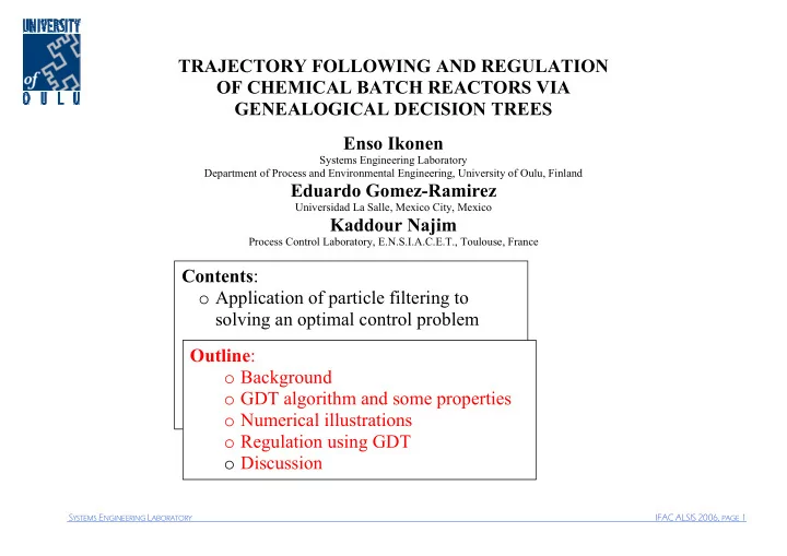
TRAJECTORY FOLLOWING AND REGULATION OF CHEMICAL BATCH REACTORS VIA GENEALOGICAL DECISION TREES Enso Ikonen Systems Engineering Laboratory Department of Process and Environmental Engineering, University of Oulu, Finland Eduardo Gomez-Ramirez Universidad La Salle, Mexico City, Mexico Kaddour Najim Process Control Laboratory, E.N.S.I.A.C.E.T., Toulouse, France Contents : o Application of particle filtering to solving an optimal control problem Outline : o Background o GDT algorithm and some properties o Numerical illustrations o Regulation using GDT o Discussion PAGE 1 S YSTEMS YSTEMS E NGINEER ING L AB ATORY IFAC ALSIS IFAC ALSIS 200 2006, 6, PAGE NGINEERING ABORATORY
BACKGROUND o Optimal filtering o Bayesian approach: Estimate the evolving posterior distribution recursively in time (prediction + updating) o Kalman filter (linear Gaussian) o Particle filtering aka Sequential Monte Carlo (non-linear non-Gaussian) o Importance Sampling & Resampling Step 0. Initialization (Set initial particle positions) Step 1. Importance Sampling • Predict (using model) • Evaluate importance weights (using observation) Step 2. Resampling (Sample from weighted distribution) o Duality between optimal filtering and regulation PAGE 2 S YSTEMS YSTEMS E NGINEER ING L AB ATORY IFAC IFAC ALSIS ALSIS 200 2006, 6, PAGE NGINEERING ABORATORY
PROBLEM FORMULATION Model: ( ) = X F X , U ; X − n n n 1 n 0 ( ) Y = h X n n n Control objective: T T 2 ( ) 2 ref = + − J U , U ,..., U U Y Y ∑ ∑ T 1 2 T n n n A B = n = n 1 n 1 n T length of trajectory (horizon) A , B control and error costs (covariances) n n Find the sequence of control actions that will minimize the control objective for open-loop control. PAGE 3 S YSTEMS YSTEMS E NGINEER ING L AB ATORY IFAC IFAC ALSIS ALSIS 200 2006, 6, PAGE NGINEERING ABORATORY
OPTIMIZATION OF THE CONTROL SEQUENCE Idea: Associate Gaussian distributions to the norms of the control actions and tracking errors, and translate the cost function as the likelihood of a conditional probability Algorithm: i ˆ X = = Initialize recursions: X , i 1 , N , n = 1. 0 0 ( ) i ~ N Generate iid controls: U 0 , A . n n ( ) ( ) i i i i i ˆ = Y = Evaluate model: X F X , U ; h X . − n n n 1 n n n n β 2 i ref − − exp Y Y n n 2 B i = N n Weight according to p . n β 2 j ref − − ∑ exp Y Y n n 2 B = j 1 n N ( ) i = δ = Resample controls from p u ∑ p for each j 1 , N n n i U = i 1 n which leads to: ( ) ( ) for each j j i i j j ˆ ˆ ˆ = = X F X , U ; Y h X . { } − n n n 1 n n n n ∈ i 1 , N = Repeat for n 2 , T . PAGE 4 S YSTEMS YSTEMS E NGINEER ING L AB ATORY IFAC IFAC ALSIS ALSIS 200 2006, 6, PAGE NGINEERING ABORATORY
GENEALOGICAL DECISION TREE Interpretation as a genetic particle evolution model j ˆ Interpret state X as the parent of − n 1 i ˆ : individual X n j i ˆ ˆ = X o denote X , etc. − n 1 , n − n 1 Ancestral lines: i i ˆ ˆ ← ← X ... U ... 0 , n 1 , n i k i k ˆ ˆ ˆ ˆ ← = ← = X X U U − − − − n 2 , n n 2 n 2 , n n 2 i j i j ˆ ˆ ˆ ˆ ← = ← = X X U U − − n 1 , n − n 1 , n − n 1 n 1 i i i i ˆ ˆ ˆ ˆ ← = ← = X X U U n , n n n , n n Solution at n = T : ( ) i i i ˆ ˆ ˆ = I arg inf J U , U ,..., U n 1 , n 2 , n n , n = i 1 , N PAGE 5 S YSTEMS YSTEMS E NGINEER ING L AB ATORY IFAC ALSIS IFAC ALSIS 200 2006, 6, PAGE NGINEERING ABORATORY
CONVERGENCE Idea : - Associate Gaussian distributions to the norms in the cost function - Translate the cost function as the likelihood of a conditional probability - Duality between control and filtering problems Corresponding filtering problem: ( ) ( ) = = + X F X , W ; Y h X V − n n n 1 n n n n n where W and V are Gaussian random vectors with covariances A n and B n . We can show the following (see works with P. Del Moral): 1. To find control actions which minimize the control objective, it is equivalent to look for most likely W. 2. The conditional probability mass of W is concentrated around the optimal control sequence: { } ( ) ( ) ref ref ∈ = = Pr W ,..., W d w ,..., w Y Y ,..., Y Y 1 n 1 n 1 1 n n − β 1 n n 2 ( ) 2 = + ref − exp w Y h X d w ... d w ∑ ∑ k k k k 1 n A Z 2 k B = = k k 1 k 1 n − β 1 ( ) = exp J w ,..., w d w ... d w n 1 n 1 n Z 2 n 3. Convergence of actions to optimal actions (as N → ∞ ). PAGE 6 S YSTEMS YSTEMS E NGINEER ING L AB ATORY IFAC ALSIS IFAC ALSIS 200 2006, 6, PAGE NGINEERING ABORATORY
NUMERICAl EXAMPLES (1) ‘ABC’-batch plant Plant 20 nonlinear equations: 15 dc ( ) 2 A = − k T c 1 A dt ref , c B dc ( ) ( ) 10 2 B = − k T c k T c T, T 1 A 2 B dt dT ( ) ( ) ( ) ( ) u 2 = γ + γ + + + + k T c k T c a a T b b T 5 1 1 A 2 2 B 1 2 1 2 dt temperature target trajectory: 0 ( ) 0 10 20 30 40 50 60 70 80 90 T ref = − 20 exp 0 . 02 t 8 GDT 6 optimize sequence of ∆ u’s A = 2 2 (‘tolerated dev. on input’) 4 u B = 0.2 2 (tolerated dev. on output’) β = 1, 2 N = 2500 (# particles) 0 0 10 20 30 40 50 60 70 80 90 Results time temperature (output) design specs fulfilled temperature reference (target) randomness apparent dimensionless scaling (input) PAGE 7 S YSTEMS YSTEMS E NGINEER ING L AB ATORY IFAC IFAC ALSIS ALSIS 200 2006, 6, PAGE NGINEERING ABORATORY
NUMERICAL EXAMPLES (2) RTP-repetitive plant Plant 1000 nonlinear equations: ( ) ( ) 800 dT 4 4 F = − − − − b u c T T c T T u 1 F P 2 F A ref dt T F , T P , T p T F ( ) dT 600 4 4 P = − c T T 3 F P dt temperature target trajectory T P 400 consisting of ramp and constant 200 phases 0 2 4 6 8 10 12 14 16 GDT 4 optimize sequence of u’s A = 1 (‘tolerated dev. on input’) 3 B = 1 (tolerated dev. on output’) 2 u β = 1, N = 500 (# particles) 1 Results 0 0 2 4 6 8 10 12 14 16 design specs fulfilled time part temperature randomness apparent heating intensity More examples available: 3x3 power plant, 2-joint robot arm, PAGE 8 S YSTEMS YSTEMS E NGINEER ING L AB ATORY IFAC ALSIS IFAC ALSIS 200 2006, 6, PAGE NGINEERING ABORATORY
GDT-BASED REGULATION Feedback: Algorithm 1. Add ( SISO linear ) feedback based on output deviation (PI, for example) off-line: • suitable, e.g., for partially measured 1. Solve optimal trajectories of length T output/state trajectories from K initial states x 0 2. Receding-horizon MPC • solve optimization problem from 2. Store all sequences. current (disturbed) state • computationally heavy => discretized on-line: 3. a) if measurement of x is available : approximation with precomputed solutions Compare state x with K *( T - T min +1) states in memory and find the closest match x *. ‘Assumptions’: Set next and future controls equal to • Accuracy can be increased by making controls in the selected solution from the discretization more dense (for non- point x * forward. chaotic plants) b) if no new measurements : • Given a minimal finite horizon T min < T , Select next control from the sequence. each sequence contains a number of optimal sub-sequences 4. Apply control to plant. • Regulation problems (=setpoint 5. Return to Step 3. trajectory) + time-invariant plants make the approach feasible PAGE 9 S YSTEMS YSTEMS E NGINEER ING L AB ATORY IFAC ALSIS IFAC ALSIS 200 2006, 6, PAGE NGINEERING ABORATORY
NUMERICAL EXAMPLE (3): van der Vusse-regulation van der Vusse CSTR : setpoint setpoint A → B → C 1.15 regulated GDT 1.15 open−loop MDP ∆ c A non-monotone ss-gain 1.13 ∆ c B 1.13 non-minimum phase dyn. 1.11 1.11 1.09 c B c B 1.09 Simulations (dbase): 1.07 isothermal simulations 1.07 RMSE=0.161779 1.05 RMSE=0.258119 T = 100 (traj. length) RMSE=0.161779 1.05 RMSE=0.121665 controlled: c B manipulated: V’/V R 0 20 40 60 80 100 0 20 40 60 80 100 GDT parameters : A = 0.5 2 , B = 0.01 2 20 20 β = 1, N = 2000 regulated GDT open−loop MDP ∆ u optimized 18 18 16 16 GDT-regulation : V’/V R V’/V R K = 300 random init. states: 14 14 c A (0)=2.126 ± 10% 12 12 c B (0)=1.09 ± 10% J T < 700, T min = 60 10 10 � finite state dbase of 8 8 5760 state entries 0 20 40 60 80 100 0 20 40 60 80 100 Open-loop GDT vs. state disturbances MDP-based optimal control Simulations (regulation): GDT regulation vs state disturbances GDT-based regulation impulse disturb. in states with input constraints 10 S YSTEMS YSTEMS E NGINEER ING L AB ATORY IFAC ALSIS IFAC ALSIS 200 2006, 6, PAGE PAGE 10 NGINEERING ABORATORY
Recommend
More recommend
Explore More Topics
Stay informed with curated content and fresh updates.
