Tracking using CONDENSATION: Conditional Density Propagation M. - PDF document
Tracking using CONDENSATION: Conditional Density Propagation M. Isard and A. Blake, CONDENSATION Conditional density propagation for visual tracking, Int. J. Computer Vision 29 (1), 1998, pp. 4-28. Goal Model-based visual tracking in
Tracking using CONDENSATION: Conditional Density Propagation M. Isard and A. Blake, CONDENSATION – Conditional density propagation for visual tracking, Int. J. Computer Vision 29 (1), 1998, pp. 4-28. Goal • Model-based visual tracking in dense clutter at near video frame rates 1
Example of CONDENSATION Algorithm Approach • Probabilistic framework for tracking objects such as curves in clutter using an iterative sampling algorithm • Model motion and shape of target • Top-down approach • Simulation instead of analytic solution 2
Probabilistic Framework • Object dynamics form a temporal Markov ( ) ( ) chain Χ − = p x p x x | | t t t t − 1 1 • Observations, z t , are independent (mutually and w.r.t process) ( ) ( ) = ∏ t − p Z x X p x X p z x 1 , | | ( | ) t − t t − t t − i = i i 1 1 1 1 • Use Bayes’ rule Notation X State vector, e.g., curve’s position and orientation Z Measurement vector, e.g., image edge locations p ( X ) Prior probability of state vector; summarizes prior domain knowledge, e.g., by independent measurements p ( Z ) Probability of measuring Z ; fixed for any given image p ( Z | X ) Probability of measuring Z given that the state is X ; compares image to expectation based on state p ( X | Z ) Probability of X given that measurement Z has occurred; called state posterior 3
Tracking as Estimation • Compute state posterior, p ( X | Z ), and select next state to be the one that maximizes this (Maximum a Posteriori (MAP) estimate) • Measurements are complex and noisy, so posterior cannot be evaluated in closed form • Particle filter (iterative sampling) idea: Stochastically approximate the state posterior with a set of N weighted particles, ( s , π ), where s is a sample state and π is its weight • Use Bayes’ rule to compute p ( X | Z ) Factored Sampling • Generate a set of samples that approximates the posterior p ( X | Z ) s = N s s ( 1 ) ( ) { ,..., } • Sample set generated from p ( X ); each sample has a weight (“probability”) p s i ( ) ( ) π = z i N � j p s ( ) ( ) z = j 1 = p z x p z x ( ) ( | ) 4
Factored Sampling N =15 X • CONDENSATION for one image Estimating Target State ����� ����� ������������� ����������������� ������������� ������������� 5
Bayes’ Rule This is what you may know a priori, or what This is what you can you can predict evaluate Z X X p p ( | ) ( ) X Z = p ( | ) Z p ( ) This is what you want. Knowing p ( X | Z ) will tell us what is the This is a constant for a most likely state X . given image CONDENSATION Algorithm 1. Select : Randomly select N particles from {s t-1(n) } based on weights π t-1(n) ; same particle may be picked multiple times ( factored sampling ) 2. Predict : Move particles according to deterministic dynamics ( drift ), then perturb individually ( diffuse ) 3. Measure : Get a likelihood for each new sample by comparing it with the image’s local appearance, i.e., based on p (z t |x t ); then update weight accordingly to obtain {(s t(n) , π t(n) )} 6
n − π n s ( ) ( ) 1 , k k − 1 Posterior at time k -1 drift diffuse Predicted state at time k ( n s ) observation k density measure Posterior at time k ( , n π n s ) ( ) k k Notes on Updating • Enforcing plausibility: Particles that represent impossible configurations are discarded • Diffusion modeled with a Gaussian • Likelihood function: Convert “goodness of prediction” score to pseudo-probability – More markings closer to predicted markings → higher likelihood 7
State Posterior ����� ����� ������������� State Posterior Animation 8
Object Motion Model • For video tracking we need a way to propagate probability densities, so we need a “motion model” such as X t +1 = A X t + B W t where W is a noise term and A and B are state transition matrices that can be learned from training sequences • The state, X , of an object, e.g., a B-spline curve, can be represented as a point in a 6D state space of possible 2D affine transformations of the object Evaluating p ( Z | X ) M � = + φ φ p z x qp z clutter p z x m p ( | ) ( | ) ( | , ) ( ) m = m 1 where φ m = {true measurement is z m } for m = 1,…, M , and q = 1 - Σ m p ( φ m ) is the probability that the target is not visible 2 − − < δ x z if x z φ = m m m m m ρ otherwise 9
Dancing Example Hand Example 10
Pointing Hand Example Glasses Example • 6D state space of affine transformations of a spline curve • Edge detector applied along normals to the spline • Autoregressive motion model 11
3D Model-based Example • 3D state space: image position + angle • Polyhedral model of object Minerva • Museum tour guide robot that used CONDENSATION to track its position in the museum Desired Location Exhibit 12
Advantages of Particle Filtering • Nonlinear dynamics, measurement model easily incorporated • Copes with lots of false positives • Multi-modal posterior okay (unlike Kalman filter) • Multiple samples provides multiple hypotheses • Fast and simple to implement 13
Recommend


More recommend
Explore More Topics
Stay informed with curated content and fresh updates.