Tomographic inversion Velocity determination with CRS attributes: - PowerPoint PPT Presentation
CO 2 CRS: Tomography T. Klver & J. Mann Introduction Tomographic inversion Velocity determination with CRS attributes: NIP waves & velocities CRS tomography Inversion procedure data extraction and preconditioning First example
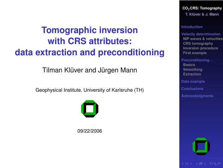
CO 2 CRS: Tomography T. Klüver & J. Mann Introduction Tomographic inversion Velocity determination with CRS attributes: NIP waves & velocities CRS tomography Inversion procedure data extraction and preconditioning First example Preconditioning. . . Basics Tilman Klüver and Jürgen Mann Smoothing Extraction Data example Conclusions Geophysical Institute, University of Karlsruhe (TH) Acknowledgments 09/22/2006
CO 2 CRS: Tomography Overview T. Klüver & J. Mann Introduction Velocity determination Introduction NIP waves & velocities CRS tomography Inversion procedure First example Velocity determination with 3D CRS attributes Preconditioning. . . Basics Smoothing Extraction Attribute preconditioning and extraction Data example Conclusions Synthetic data example Acknowledgments Conclusions Acknowledgments
CO 2 CRS: Tomography Introduction T. Klüver & J. Mann Introduction Velocity determination Construction of a background/migration velocity model NIP waves & velocities CRS tomography is one of the key aims of seismic imaging schemes. Inversion procedure First example Preconditioning. . . Basics ◮ Problems with conventional reflection tomography: Smoothing Extraction identifying and picking events in the prestack data Data example ◮ 3D velocity models for depth imaging Conclusions Acknowledgments ◮ Tomographic approach based on CRS stack results ◮ Advantages: ◮ picking in simulated ZO volume of high S/N ratio ◮ pick locations independent of each other ◮ very few picks required
CO 2 CRS: Tomography NIP waves and velocities T. Klüver & J. Mann ( M h p ξ , ) T , , ξ ξ Introduction ξ ξ ξ Velocity determination NIP waves & velocities CRS tomography Inversion procedure First example Preconditioning. . . Basics Smoothing Extraction Data example Conclusions NIP Acknowledgments CRS attributes M h and p ξ at ( t 0 , ξ ξ ξ ) describe second-order traveltime approximation of emerging NIP wave.
CO 2 CRS: Tomography NIP waves and velocities T. Klüver & J. Mann ( M h p ξ , ) T , , ξ ξ Introduction ξ ξ ξ Velocity determination NIP waves & velocities CRS tomography Inversion procedure First example Preconditioning. . . Basics Smoothing Extraction Data example Conclusions NIP Acknowledgments In consistent velocity models, NIP waves focus at zero traveltime.
CO 2 CRS: Tomography Tomography with CRS attributes T. Klüver & J. Mann Introduction Velocity determination NIP waves & velocities CRS tomography Inversion procedure First example Find a velocity model in which all considered NIP Preconditioning. . . waves, described by kinematic wavefield attributes, Basics Smoothing are correctly modeled. Extraction Data example For tomographic inversion in 3D, one azimuth φ of Conclusions M h is required: M φ . Acknowledgments For multi-azimuth data the full Matrix M h is to be preferred.
CO 2 CRS: Tomography 3D tomography with CRS attributes T. Klüver & J. Mann Introduction Data and model components Velocity determination NIP waves & velocities CRS tomography Inversion procedure (p ,p ) M First example ξ ξ ξ ξ y x τ Preconditioning. . . (ξ ,ξ ) Basics Smoothing x y Extraction Data example Conclusions v(x,y,z) (e ,e ) Acknowledgments x y (x,y,z) NIP Data: Model: ( τ , M 11 , M 12 , M 22 , ( x , y , z , e x , e y ) i , v jkl p ξ x , p ξ y , ξ x , ξ y ) i v jkl : B-spline τ = t 0 / 2 coefficients
CO 2 CRS: Tomography Inversion procedure T. Klüver & J. Mann Introduction Velocity determination NIP waves & velocities ◮ nonlinear least-squares problem: CRS tomography Inversion procedure ◮ iterative solution, local linearization First example ◮ τ , p ξ x , p ξ y , ξ x , ξ y Preconditioning. . . Basics from kinematic ray tracing Smoothing ◮ M h = DB − 1 from dynamic ray-tracing: Extraction � � A B Data example T = C D Conclusions propagator matrix in Cartesian coordinates Acknowledgments ◮ model update ∆ m : least-squares solution of F ∆ m = ∆ d ◮ calculation of Fréchet derivatives (matrix F ): ray perturbation theory
CO 2 CRS: Tomography Regularization/additional constraints T. Klüver & J. Mann Introduction Velocity determination NIP waves & velocities CRS tomography Inversion procedure Regularization: First example Preconditioning. . . ◮ minimization of second derivatives of velocity Basics Smoothing (spatially dependent) Extraction Data example Additional constraints: Conclusions ◮ v ( x , y , z ) values at arbitrary locations ( x , y , z ) Acknowledgments ◮ force velocity structure to follow local reflector structure
CO 2 CRS: Tomography Synthetic example: T. Klüver & J. Mann forward modeled attributes Introduction Velocity determination NIP waves & velocities CRS tomography Inversion procedure First example Model description: Preconditioning. . . Basics ◮ 9 × 9 × 9 = 729 B-spline knots Smoothing Extraction ◮ horizontal spacing: 500 m Data example Conclusions ◮ vertical spacing: 400 m Acknowledgments ◮ 1008 NIP-locations used to model the input data ◮ initial ray direction follows local velocity gradient
True model Inversion result CO 2 CRS: Tomography y [m] y [m] T. Klüver & J. Mann 0 1000 2000 3000 4000 5000 0 1000 2000 3000 4000 5000 0 0 4500 4500 4000 4000 1000 1000 Introduction velocity [m/s] velocity [m/s] 3500 3500 z [m] z [m] Velocity determination 2000 3000 2000 3000 NIP waves & velocities 2500 2500 3000 3000 CRS tomography 2000 2000 Inversion procedure 1500 1500 First example x=0m x=0m Preconditioning. . . y [m] y [m] 0 1000 2000 3000 4000 5000 0 1000 2000 3000 4000 5000 Basics 0 0 4500 4500 Smoothing 4000 4000 Extraction 1000 1000 velocity [m/s] velocity [m/s] 3500 3500 Data example z [m] z [m] 2000 3000 2000 3000 2500 2500 Conclusions 3000 3000 2000 2000 Acknowledgments 1500 1500 x=2000m x=2000m y [m] y [m] 0 1000 2000 3000 4000 5000 0 1000 2000 3000 4000 5000 0 0 4500 4500 4000 4000 1000 1000 velocity [m/s] velocity [m/s] 3500 3500 z [m] z [m] 2000 3000 2000 3000 2500 2500 3000 3000 2000 2000 1500 1500 x=4000m x=4000m
Difference Inversion result CO 2 CRS: Tomography y [m] y [m] T. Klüver & J. Mann 0 1000 2000 3000 4000 5000 0 1000 2000 3000 4000 5000 0 0 300 4500 200 4000 1000 1000 Introduction velocity [m/s] velocity [m/s] 100 3500 z [m] z [m] Velocity determination 2000 0 2000 3000 NIP waves & velocities -100 2500 3000 3000 CRS tomography -200 2000 Inversion procedure -300 1500 First example x=0m x=0m Preconditioning. . . y [m] y [m] 0 1000 2000 3000 4000 5000 0 1000 2000 3000 4000 5000 Basics 0 0 300 4500 Smoothing 200 4000 Extraction 1000 1000 velocity [m/s] velocity [m/s] 100 3500 Data example z [m] z [m] 2000 0 2000 3000 -100 2500 Conclusions 3000 3000 -200 2000 Acknowledgments -300 1500 x=2000m x=2000m y [m] y [m] 0 1000 2000 3000 4000 5000 0 1000 2000 3000 4000 5000 0 0 300 4500 200 4000 1000 1000 velocity [m/s] velocity [m/s] 100 3500 z [m] z [m] 2000 0 2000 3000 -100 2500 3000 3000 -200 2000 -300 1500 x=4000m x=4000m
CO 2 CRS: Tomography Motivation T. Klüver & J. Mann Introduction Velocity determination CRS attributes have characteristic features: NIP waves & velocities CRS tomography ◮ they should be constant along the wavelet Inversion procedure First example ◮ they should vary smoothly along the event Preconditioning. . . Basics However, in practice Smoothing Extraction ◮ unphysical fluctuations Data example Conclusions ◮ outliers Acknowledgments ◮ possibly not locally coherent Thus ◮ event-consistent smoothing ◮ identification of valid pick locations
Recommend
More recommend
Explore More Topics
Stay informed with curated content and fresh updates.
