Time Series Mining and Forecasting Duen Horng (Polo) Chau Georgia - PowerPoint PPT Presentation
CSE 6242 / CX 4242 Time Series Mining and Forecasting Duen Horng (Polo) Chau Georgia Tech Slides based on Prof. Christos Faloutsoss materials Outline Motivation Similarity search distance functions Linear
CSE 6242 / CX 4242 Time Series Mining and Forecasting Duen Horng (Polo) Chau Georgia Tech Slides based on Prof. Christos Faloutsos’s materials
Outline • Motivation • Similarity search – distance functions • Linear Forecasting • Non-linear forecasting • Conclusions
Problem definition • Given : one or more sequences x 1 , x 2 , … , x t , … ( y 1 , y 2 , … , y t , …) (… ) • Find – similar sequences; forecasts – patterns; clusters; outliers
Motivation - Applications • Financial, sales, economic series • Medical – ECGs +; blood pressure etc monitoring – reactions to new drugs – elderly care
Motivation - Applications (cont’d) • ‘Smart house’ – sensors monitor temperature, humidity, air quality • video surveillance
Motivation - Applications (cont’d) • Weather, environment/anti-pollution – volcano monitoring – air/water pollutant monitoring
Motivation - Applications (cont’d) • Computer systems – ‘Active Disks’ (buffering, prefetching) – web servers (ditto) – network traffic monitoring – ...
Stream Data: Disk accesses #bytes time
Problem #1: Goal: given a signal (e.g.., #packets over time) Find: patterns, periodicities, and/or compress lynx caught per year (packets per day; count temperature per day) year
Problem#2: Forecast Given x t , x t-1 , …, forecast x t+1 90 Number of packets sent 80 70 60 ?? 50 40 30 20 10 0 1 3 5 7 9 11 Time Tick
Problem#2’: Similarity search E.g.., Find a 3-tick pattern, similar to the last one 90 Number of packets sent 80 70 60 ?? 50 40 30 20 10 0 1 3 5 7 9 11 Time Tick
Problem #3: • Given: A set of correlated time sequences • Forecast ‘Sent(t)’ 90 sent 68 Number of packets lost repeated 45 23 0 1 4 6 9 11 Time Tick
Important observations Patterns, rules, forecasting and similarity indexing are closely related: • To do forecasting, we need – to find patterns/rules – to find similar settings in the past • to find outliers, we need to have forecasts – (outlier = too far away from our forecast)
Outline • Motivation • Similarity Search and Indexing • Linear Forecasting • Non-linear forecasting • Conclusions
Outline • Motivation • Similarity search and distance functions – Euclidean – Time-warping • ...
Importance of distance functions Subtle, but absolutely necessary : • A ‘must’ for similarity indexing (-> forecasting) • A ‘must’ for clustering Two major families – Euclidean and Lp norms – Time warping and variations
Euclidean and Lp x(t) y(t) ! ! n 2 D ( x , y ) ( x y ) ∑ = − i i i 1 = ... ! ! n p L ( x , y ) | x y | ∑ = − p i i i 1 = •L 1 : city-block = Manhattan •L 2 = Euclidean •L ∞
Observation #1 • Time sequence -> n-d vector Day-n Day-2 ... Day-1
Observation #2 Day-n Euclidean distance is Day-2 closely related to ... – cosine similarity – dot product Day-1 – ‘cross-correlation’ function
Time Warping • allow accelerations - decelerations – (with or w/o penalty) • THEN compute the (Euclidean) distance (+ penalty) • related to the string-editing distance
Time Warping ‘stutters’:
Time warping Q: how to compute it? A: dynamic programming D( i, j ) = cost to match prefix of length i of first sequence x with prefix of length j of second sequence y
Time warping Thus, with no penalty for stutter, for sequences x 1 , x 2 , …, x i,; y 1 , y 2 , …, y j no stutter D ( i 1 , j 1 ) − − $ ! x-stutter D ( i , j ) x [ i ] y [ j ] min D ( i , j 1 ) = − + − # ! D ( i 1 , j ) y-stutter − "
Time warping VERY SIMILAR to the string-editing distance no stutter D ( i 1 , j 1 ) − − $ ! x-stutter D ( i , j ) x [ i ] y [ j ] min D ( i , j 1 ) = − + − # ! D ( i 1 , j ) y-stutter − "
Time warping • Complexity: O(M*N) - quadratic on the length of the strings • Many variations (penalty for stutters; limit on the number/percentage of stutters; …) • popular in voice processing [Rabiner + Juang]
Other Distance functions • piece-wise linear/flat approx.; compare pieces [Keogh+01] [Faloutsos+97] • ‘cepstrum’ (for voice [Rabiner+Juang]) – do DFT; take log of amplitude; do DFT again! • Allow for small gaps [Agrawal+95] See tutorial by [Gunopulos + Das, SIGMOD01]
Other Distance functions • In [Keogh+, KDD’04]: parameter-free, MDL based
Conclusions Prevailing distances: – Euclidean and – time-warping
Outline • Motivation • Similarity search and distance functions • Linear Forecasting • Non-linear forecasting • Conclusions
Linear Forecasting
Forecasting “Prediction is very difficult, especially about the future.” - Nils Bohr Danish physicist and Nobel Prize laureate
Outline • Motivation • ... • Linear Forecasting – Auto-regression: Least Squares; RLS – Co-evolving time sequences – Examples – Conclusions
Reference [Yi+00] Byoung-Kee Yi et al.: Online Data Mining for Co-Evolving Time Sequences , ICDE 2000. (Describes MUSCLES and Recursive Least Squares)
Problem#2: Forecast • Example: give x t-1 , x t-2 , …, forecast x t 90 Number of packets sent 80 70 60 ?? 50 40 30 20 10 0 1 3 5 7 9 11 Time Tick
Forecasting: Preprocessing MANUALLY: remove trends spot periodicities 7 days 3 6 2 5 2 3 1 2 0 0 1 3 5 7 9 11 13 1 2 3 4 5 6 7 8 9 10 time time
Problem#2: Forecast • Solution: try to express x t as a linear function of the past: x t-1 , x t-2 , …, (up to a window of w ) Formally: 90 80 70 60 ?? 50 40 30 20 10 0 1 3 5 7 9 11 Time Tick
(Problem: Back-cast; interpolate) • Solution - interpolate: try to express x t as a linear function of the past AND the future: x t+1 , x t+2 , … x t+wfuture; x t-1 , … x t-wpast (up to windows of w past , w future ) • EXACTLY the same algo’s ?? 90 80 70 60 50 40 30 20 10 0 1 3 5 7 9 11 Time Tick
Linear Regression: idea 85 Body height patient weight height 80 75 1 27 43 70 2 43 54 65 60 3 54 72 55 … … … 50 45 25 N ?? 40 15 25 35 45 Body weight • express what we don’t know (= “dependent variable”) • as a linear function of what we know (= “independent variable(s)”)
Linear Regression: idea 85 Body height patient weight height 80 75 1 27 43 70 2 43 54 65 60 3 54 72 55 … … … 50 45 25 N ?? 40 15 25 35 45 Body weight • express what we don’t know (= “dependent variable”) • as a linear function of what we know (= “independent variable(s)”)
Linear Regression: idea 85 Body height patient weight height 80 75 1 27 43 70 2 43 54 65 60 3 54 72 55 … … … 50 45 25 N ?? 40 15 25 35 45 Body weight • express what we don’t know (= “dependent variable”) • as a linear function of what we know (= “independent variable(s)”)
Linear Regression: idea 85 Body height patient weight height 80 75 1 27 43 70 2 43 54 65 60 3 54 72 55 … … … 50 45 25 N ?? 40 15 25 35 45 Body weight • express what we don’t know (= “dependent variable”) • as a linear function of what we know (= “independent variable(s)”)
Linear Auto Regression: Time Packets Packets Sent (t-1) Sent(t) 1 - 43 2 43 54 3 54 72 … … … 25 N ??
Linear Auto Regression: Time Packets Packets ‘lag-plot’ Sent (t-1) Sent(t) 1 - 43 2 43 54 #packets sent 3 54 72 at time t … … … 25 N ?? #packets sent at time t-1 • lag w = 1 • Dependent variable = # of packets sent (S [t]) • Independent variable = # of packets sent (S[t-1])
Linear Auto Regression: Time Packets Packets ‘lag-plot’ Sent (t-1) Sent(t) 1 - 43 2 43 54 #packets sent 3 54 72 at time t … … … 25 N ?? #packets sent at time t-1 • lag w = 1 • Dependent variable = # of packets sent (S [t]) • Independent variable = # of packets sent (S[t-1])
Linear Auto Regression: Time Packets Packets ‘lag-plot’ Sent (t-1) Sent(t) 1 - 43 2 43 54 #packets sent 3 54 72 at time t … … … 25 N ?? #packets sent at time t-1 • lag w = 1 • Dependent variable = # of packets sent (S [t]) • Independent variable = # of packets sent (S[t-1])
Linear Auto Regression: Time Packets Packets ‘lag-plot’ Sent (t-1) Sent(t) 1 - 43 2 43 54 #packets sent 3 54 72 at time t … … … 25 N ?? #packets sent at time t-1 • lag w = 1 • Dependent variable = # of packets sent (S [t]) • Independent variable = # of packets sent (S[t-1])
Outline • Motivation • ... • Linear Forecasting – Auto-regression: Least Squares; RLS – Co-evolving time sequences – Examples – Conclusions
More details: • Q1: Can it work with window w > 1? • A1: YES! x t x t-1 x t-2
Recommend
More recommend
Explore More Topics
Stay informed with curated content and fresh updates.
