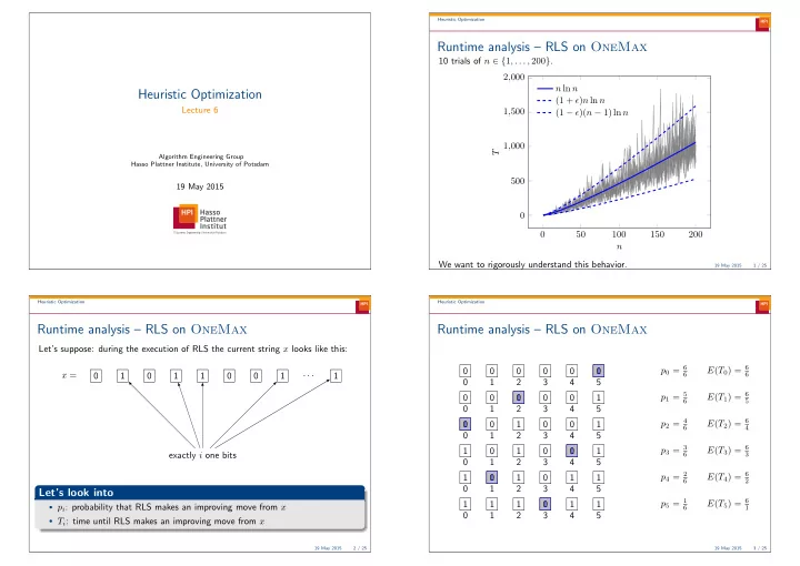
Runtime analysis RLS on OneMax 10 trials of n { 1 , . . . , 200 } . - PowerPoint PPT Presentation

Heuristic Optimization Runtime analysis – RLS on OneMax 10 trials of n ∈ { 1 , . . . , 200 } . 2 , 000 n ln n Heuristic Optimization (1 + ǫ ) n ln n Lecture 6 1 , 500 (1 − ǫ )( n − 1) ln n 1 , 000 T Algorithm Engineering Group Hasso Plattner Institute, University of Potsdam 500 19 May 2015 0 0 50 100 150 200 n We want to rigorously understand this behavior. 19 May 2015 1 / 25 Heuristic Optimization Heuristic Optimization Runtime analysis – RLS on OneMax Runtime analysis – RLS on OneMax Let’s suppose: during the execution of RLS the current string x looks like this: p 0 = 6 E ( T 0 ) = 6 0 0 0 0 0 1 0 x = · · · 0 1 0 1 1 0 0 1 1 6 6 0 1 2 3 4 5 p 1 = 5 E ( T 1 ) = 6 0 0 1 0 0 0 1 6 5 0 1 2 3 4 5 p 2 = 4 E ( T 2 ) = 6 0 1 0 1 0 0 1 6 4 0 1 2 3 4 5 p 3 = 3 E ( T 3 ) = 6 1 0 1 0 0 1 1 exactly i one bits 6 3 0 1 2 3 4 5 p 4 = 2 E ( T 4 ) = 6 1 1 0 1 0 1 1 6 2 0 1 2 3 4 5 Let’s look into p 5 = 1 E ( T 5 ) = 6 1 1 1 0 1 1 1 • p i : probability that RLS makes an improving move from x 6 1 0 1 2 3 4 5 • T i : time until RLS makes an improving move from x 19 May 2015 2 / 25 19 May 2015 3 / 25

Heuristic Optimization Heuristic Optimization Runtime analysis – RLS on OneMax Runtime analysis – RLS on OneMax Runtime p 0 = n E ( T 0 ) = n · · · 0 0 1 0 0 0 n n n 0 1 2 3 T is the random variable that counts the number of steps (function evaluations) taken by RLS until the optimum is generated. p 1 = n − 1 n · · · E ( T 1 ) = 1 0 0 1 0 0 n n − 1 n 0 1 2 3 p 2 = n − 2 n · · · E ( T 2 ) = 1 0 1 1 0 0 n n − 2 n 0 1 2 3 . . . . . . . . . . . . . . E ( T ) = E ( T 0 ) + E ( T 1 ) + · · · + E ( T 5 ) . . . . . . . = 1 /p 0 + 1 /p 1 + · · · + 1 /p 5 p n − 1 = 1 E ( T n − 1 ) = n · · · 1 1 0 1 1 1 5 5 6 n 1 1 6 1 n � � � 0 1 2 3 = = i + 1 = 6 i = 6 · 2 . 45 = 14 . 7 p i i =0 i =0 i =1 remaining zero 19 May 2015 4 / 25 19 May 2015 5 / 25 Heuristic Optimization Heuristic Optimization Coupon collector process Coupon collector process: concentration bounds Suppose there are n different kinds of coupons. We must collect all n What is the probability that T > n ln n + O ( n ) ? coupons during a series of trials. Theorem (Coupon collector upper bound) In each trial, exactly one of the n coupons is drawn, each one equally Let T be the number of trials until all n coupons are collected. Then likely. We must keep drawing in each trial until we have collected each coupon at least once. Pr( T ≥ (1 + ǫ ) n ln n ) ≤ n − ǫ Starting with zero coupons, what is the exact number of trials needed Proof. before we have all n coupons? Probability of choosing a specific coupon: 1 /n . Probability of not choosing a specific coupon: 1 − 1 /n . Theorem (Coupon collector theorem) Probability of not choosing a specific coupon for t rounds: (1 − 1 /n ) t Probability that one of the n coupons is not chosen in t rounds: n · (1 − 1 /n ) t Let T be the number of trials until all n coupons are collected. Then (union bound) n − 1 n − 1 n − 1 Let t = cn ln n , 1 n 1 � � � E ( T ) = = n − i = n p i +1 i Pr( T ≥ cn ln n ) ≤ n (1 − 1 /n ) cn ln n ≤ ne − c ln n = n · n − c = n − c +1 i =0 i =0 i =0 = n · H n = n (log n + Θ(1)) = n log n + O ( n ) 19 May 2015 6 / 25 19 May 2015 7 / 25

Heuristic Optimization Heuristic Optimization Coupon collector process: concentration bounds Runtime analysis – RLS on OneMax 2 , 000 n ln n Theorem (Coupon collector lower bound) (Doerr, 2011) (1 + ǫ ) n ln n Let T be the number of trials until all n coupons are collected. Then 1 , 500 (1 − ǫ )( n − 1) ln n Pr( T < (1 − ǫ )( n − 1) ln n ) ≤ e − n ǫ 1 , 000 T Corollary 500 Let T be the time for RLS to optimize OneMax . Then, E ( T ) = Θ( n log n ) 0 Pr( T ≥ (1 + ǫ ) n ln n ) ≤ n − ǫ 0 50 100 150 200 Pr( T < (1 − ǫ )( n − 1) ln n ) ≤ e − n − ǫ n What about (1+1) EA ? Can we use Coupon Collector? Why/why not? 19 May 2015 8 / 25 19 May 2015 9 / 25 Heuristic Optimization Heuristic Optimization Fitness levels Fitness levels A 7 Observation: fitness during optimization is always monotone increasing A 6 Pr( (1+1) EA leaves A i ) ≥ s i A 5 Idea: partition the search space { 0 , 1 } n into m sets A 1 , . . . A m such that A 4 fitness 1. ∀ i � = j : A i ∩ A j = ∅ A 3 2. � m i =1 A i = { 0 , 1 } n Law of total probability: A 2 3. for all points a ∈ A i and b ∈ A j , f ( a ) < f ( b ) if i < j E ( X ) = � F Pr( F ) E ( X | F ) A 1 We require A m to contain only optimal search points • p ( A i ) be the probability that a random chosen point belongs to A i • s i be the probability to leave level A i for level A j with j > i Procedure: for each level A i , bound the probability of leaving a level A i for a � 1 � 1 m − 1 m − 1 higher level A j , j > i . 1 � 1 � 1 � � E ( T ) ≤ p ( A i ) · + · · · + ≤ + · · · + = s i s m − 1 s 1 s m − 1 s i i =1 i =1 Figure adapted from D. Sudholt, Tutorial 2011 19 May 2015 10 / 25 19 May 2015 11 / 25

Heuristic Optimization Heuristic Optimization Runtime analysis – (1+1) EA on OneMax Runtime analysis – (1+1) EA on OneMax Theorem The expected runtime of the (1+1) EA on OneMax is O ( n log n ) . Proof We partition { 0 , 1 } n into disjoint sets A 0 , A 1 , . . . , A n where x is in A i if and only This gives only an upper bound. Maybe the (1+1) EA can be much quicker. For if it has i zeros ( n − i ones). example it could be O ( n ) or even something like O ( n log log n ) . To escape A i , it suffices to flip a single zero and leave all other bits unchanged. � n − 1 ≥ Thus, s i ≥ i 1 − 1 i s i ≤ en 1 � en , and i . n n We conclude m − 1 n 1 en � � E ( T ) ≤ ≤ i = en · H n = O ( n log n ) . s i i =1 i =1 19 May 2015 12 / 25 19 May 2015 13 / 25 Heuristic Optimization Heuristic Optimization Runtime analysis – (1+1) EA on OneMax Runtime analysis – (1+1) EA on OneMax Proof of Lemma. The initial solution has at most n/ 2 one bits with probability at least 1 / 2 . There is a constant probability that in ( n − 1) ln n steps one of the remaining zero bits does not flip: Theorem (Droste, Jansen, Wegener 2002) • Probability a particular bit doesn’t flip in t steps: (1 − 1 /n ) t The expected runtime of the (1+1) EA on OneMax is Ω( n log n ) . • Probability it flips at least once in t steps: 1 − (1 − 1 /n ) t • Probability n/ 2 bits flip at least once in t steps: (1 − (1 − 1 /n ) t ) n/ 2 • Probability at least one of the n/ 2 bits does not flip in t steps: 1 − [1 − (1 − 1 /n ) t ] n/ 2 . Set t = ( n − 1) ln n . Then Lemma 1 − [1 − (1 − 1 /n ) t ] n/ 2 = 1 − [1 − (1 − 1 /n ) ( n − 1) ln n ] n/ 2 The probability that the (1+1) EA needs at least ( n − 1) ln n steps is at least a constant c . ≥ 1 − [1 − (1 /e ) ln n ] n/ 2 = 1 − [1 − 1 /n ] n/ 2 = 1 − [1 − 1 /n ] n · 1 / 2 ≥ (1 − (2 e )) − 1 / 2 = c. 19 May 2015 14 / 25 19 May 2015 15 / 25

Heuristic Optimization Heuristic Optimization Runtime analysis – (1+1) EA on OneMax Fitness levels There are several more advanced results that use the fitness levels Theorem (Droste, Jansen, Wegener 2002) technique: The expected runtime of the (1+1) EA on OneMax is Ω( n log n ) . Proof Expected runtime of the (1+ λ ) EA on LeadingOnes is O ( λn + n 2 ) (Jansen et al., 2005) Expected runtime: Expected runtime of the ( µ +1) EA on LeadingOnes is O ( µn log n + n 2 ) (Witt, ∞ � E ( T ) = t Pr( T = t ) ≥ ( n − 1) ln n · Pr( T ≥ ( n − 1) ln n ) 2006) t =1 ≥ ( n − 1) ln n · c = Ω( n log n ) . Fitness levels for proving lower bounds (Sudholt, 2010). by previous lemma Non-elitist populations (Lehre, 2011). Upper bound given by fitness levels is tight. 19 May 2015 16 / 25 19 May 2015 17 / 25 Heuristic Optimization Heuristic Optimization Drift Analysis Drift Analysis – Deterministic Process Consider a process moving towards/away from a goal (possibly stochastically). Consider a process that moves as follows. In each step, Model this as a sequence of numbers X 0 , X 1 , . . . where • With probability 1 , move one step toward the goal. X t := distance from the goal at time t. � 0 if X t = 0 Starting at distance n , how many steps until the goal is reached? n E ( X t − X t +1 ) = (10 , 9 , 8 , 7 , 6 , 5 , 4 , 3 , 2 , 1 , 0) 1 otherwise (10 , 9 , 8 , 9 , 8 , 7 , 6 , 5 , 4 , 5 , . . . , 0) ??? Drift is E ( X t − X t +1 ) = 1 as long as X t > 0 . Definition Expected time to reach the goal: The drift of a process at time t is the expected decrease in distance from a goal: E ( T ) = maximum distance = n E ( X t − X t +1 ) 1 = n. drift Drift analysis allows us to relate the drift to the time to reach the goal . 19 May 2015 18 / 25 19 May 2015 19 / 25