Time-Series Data Numerical data obtained at regular time intervals - PowerPoint PPT Presentation

Time-Series Data  Numerical data obtained at regular time intervals  The time intervals can be annually, quarterly, daily, hourly, etc.  Example: Year: 1999 2000 2001 2002 2003 Sales: 75.3 74.2 78.5 79.7 80.2

Time-Series Plot A time-series plot is a two-dimensional plot of time series data  the vertical axis U.S. Inflation Rate measures the 16.00 variable of interest 14.00 Inflation Rate (%) 12.00 10.00 8.00  the horizontal axis 6.00 corresponds to the 4.00 2.00 time periods 0.00 1975 1977 1979 1981 1983 1985 1987 1989 1991 1993 1995 1997 1999 2001 Year

Time Series Example

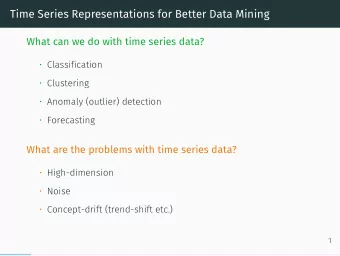
Mining Time Series Data  Prediction and Forecasting  Similarity Search

The Importance of Forecasting  Governments forecast unemployment, interest rates, and expected revenues from income taxes for policy purposes  Marketing executives forecast demand, sales, and consumer preferences for strategic planning  College administrators forecast enrollments to plan for facilities and for faculty recruitment  Traders forecast stock prices, interest rates and volatilities to make profit

Time-Series Components Time Series Trend Seasonal Cyclical Irregular Component Component Component Component

Trend Component  Long-run increase or decrease over time (overall upward or downward movement)  Data taken over a long period of time Sales Time

Trend Component  Trend can be upward or downward  Trend can be linear or non-linear Sales Sales Time Time Downward linear trend Upward nonlinear trend

Seasonal Component  Short-term regular wave-like patterns  Observed within 1 year  Often monthly or quarterly Sales Summer Winter Summer Fall Spring Winter Fall Spring Time (Quarterly)

Cyclical Component  Long-term wave-like patterns  Regularly occur but may vary in length  Often measured peak to peak/trough to trough 1 Cycle Sales Year

Irregular Component  Unpredictable, random, “residual” fluctuations  Due to random variations of  Nature  Accidents or unusual events  “Noise” in the time series

Additive Time-Series Model  Used primarily for forecasting     Y T S C I i i i i i where T i = Trend value at time i S i = Seasonal value at time i C i = Cyclical value at time i I i = Irregular (random) value at time i

Multiplicative Time-Series Model  Used primarily for forecasting     Y T S C I i i i i i where T i = Trend value at time i S i = Seasonal value at time i C i = Cyclical value at time i I i = Irregular (random) value at time i

Forecasting Time Series  Smoothing-based forecasting (moving average)  Trend based forecasting  Autoregressive models  Many alternative models exist

Moving Averages  Calculate moving averages to get an overall impression of the pattern of movement over time Moving Average: averages of consecutive time series values for a chosen period of length L

Moving Averages  Used for smoothing  A series of arithmetic means over time  Result dependent upon choice of L (length of period for computing means)  Examples:  For a 5 year moving average, L = 5  For a 7 year moving average, L = 7  Etc.

Moving Averages  Example: Five-year moving average  First average:     Y Y Y Y Y 1 2 3 4 5  MA(5) 5  Second average:     Y Y Y Y Y 2 3 4 5 6  MA(5) 5  etc.

Example: Annual Data Year Sales Annual Sales 1 23 60 2 40 50 3 25 … 40 4 27 Sales 5 32 30 6 48 20 7 33 10 8 37 … 0 9 37 1 2 3 4 5 6 7 8 9 10 11 10 50 Year 11 40 etc… etc…

Calculating Moving Averages 5-Year Average Moving Year Sales Year Average     1 2 3 4 5  1 23 3 3 29.4 5 2 40 4 34.4     23 40 25 27 32 3 25 5 33.0  29.4 5 4 27 6 35.4 5 32 7 37.4 6 48 8 41.0 7 33 9 39.4 8 37 … … 9 37  Each moving average is for a 10 50 consecutive block of 5 years 11 40

Annual vs. Moving Average  The 5-year Annual vs. 5-Year Moving Average moving average 60 smoothes the 50 data and shows 40 the underlying Sales 30 trend 20 10 0 1 2 3 4 5 6 7 8 9 10 11 Year Annual 5-Year Moving Average

Exponential Smoothing  A weighted moving average  Weights decline exponentially  Most recent observation weighted most  Used for smoothing and short term forecasting (often one period into the future )

Exponential Smoothing  The weight (smoothing coefficient) is W  Subjectively chosen  Range from 0 to 1  Smaller W gives more smoothing, larger W gives less smoothing

Exponential Smoothing Model E  Y For i = 2, 3, 4, … 1 1    E WY (1 W)E  i i i 1 where: E i = exponentially smoothed value for period i E i-1 = exponentially smoothed value already computed for period i - 1 Y i = observed value in period i W = weight (smoothing coefficient), 0 < W < 1

Exponential Smoothing Example  Suppose we use weight W = .2 Time Forecast Sales Exponentially Smoothed Period from prior (Y i ) Value for this period (E i ) (i) period (E i-1 ) E 1 = Y 1 1 23 -- 23 since no 2 40 23 (.2)(40)+(.8)(23)=26.4 prior 3 25 26.4 (.2)(25)+(.8)(26.4)=26.12 information 4 27 26.12 (.2)(27)+(.8)(26.12)=26.296 exists 5 32 26.296 (.2)(32)+(.8)(26.296)=27.437  E 6 48 27.437 (.2)(48)+(.8)(27.437)=31.549 i   WY (1 W)E 7 33 31.549 (.2)(48)+(.8)(31.549)=31.840  i i 1 8 37 31.840 (.2)(33)+(.8)(31.840)=32.872 9 37 32.872 (.2)(37)+(.8)(32.872)=33.697 10 50 33.697 (.2)(50)+(.8)(33.697)=36.958 etc. etc. etc. etc.

Sales vs. Smoothed Sales  Fluctuations have been smoothed 60 50  NOTE: the 40 smoothed value in Sales 30 this case is 20 generally a little 10 low, since the trend is upward sloping 0 1 2 3 4 5 6 7 8 9 10 and the weighting Time Period factor is only .2 Sales Smoothed

Forecasting Time Period i + 1  The smoothed value in the current period (i) is used as the forecast value for next period (i + 1) : ˆ  Y E  i 1 i

Trend-Based Forecasting  Estimate a trend line using regression analysis  Use time(X) as the Time Sales independent variable : Period Year (Y) (X) ˆ 1999 0 20  0  Y b b X 1 2000 1 40 2001 2 30 2002 3 50 2003 4 70 2004 5 65

Trend-Based Forecasting  The linear trend forecasting Time equation is: Period Sales Year ˆ   Y 21.905 9.5714 X (X) (Y) i i 1999 0 20 Sales trend 2000 1 40 80 2001 2 30 70 60 50 2002 3 50 sales 40 30 2003 4 70 20 10 2004 5 65 0 0 1 2 3 4 5 6 Year

Trend-Based Forecasting  Forecast for time period 6: Time ˆ   Y 21.905 9.5714 (6) Period Year Sales (X)  79.33 (Y) 1999 0 20 Sales trend 2000 1 40 80 2001 2 30 70 60 2002 3 50 50 sales 40 2003 4 70 30 2004 5 65 20 10 2005 6 ?? 0 0 1 2 3 4 5 6 Year

Nonlinear Trend Forecasting  A nonlinear regression model can be used when the time series exhibits a nonlinear trend  Quadratic form is one type of a nonlinear model: 2     Y β β X β X ε i 0 1 2 i i i  Can try other functional forms to get best fit

Model Selection Using Differences  Use a linear trend model if the first differences are approximately constant Why ?       (Y Y Y Y Y Y ) ( ) ( )  2 1 3 2 n n - 1  Use a quadratic trend model if the second differences are approximately constant        [(Y Y ) ( Y Y )] [(Y Y ) ( Y Y )] 3 2 2 1 4 3 3 2      [(Y Y ) ( Y Y )]  n n - 1 n - 1 n - 2

Autoregressive Models  Used for forecasting  Takes advantage of autocorrelation  1st order - correlation between consecutive values  2nd order - correlation between values 2 periods apart  p th order Autoregressive models:        Y A A Y A Y A Y δ  i 0 1 i - 1 2 i - 2 p i - p i Random Error

Autoregressive Model: Example The Office Concept Corp. has acquired a number of office units (in thousands of square feet) over the last eight years. Develop the second order Autoregressive model. Year Units 97 4 98 3 99 2 00 3 01 2 02 2 03 4 04 6     Y A A Y A Y δ i 0 1 i - 1 2 i - 2 i

Autoregressive Model: Example Solution Year Y i Y i-1 Y i-2  Develop the 2nd order 97 4 -- -- table 98 3 4 --  Build a regression model 99 2 3 4 00 3 2 3 Model Output 01 2 3 2 02 2 2 3 Coefficients 03 4 2 2 Intercept 3.5 04 6 4 2 X Variable 1 0.8125 X Variable 2 -0.9375     Y A A Y A Y δ i 0 1 i - 1 2 i - 2 i ˆ     Y 3.5 0.8125Y 0.9375Y i  i 1 i 2