This Lecture Classification Machine Learning and Pattern - PowerPoint PPT Presentation

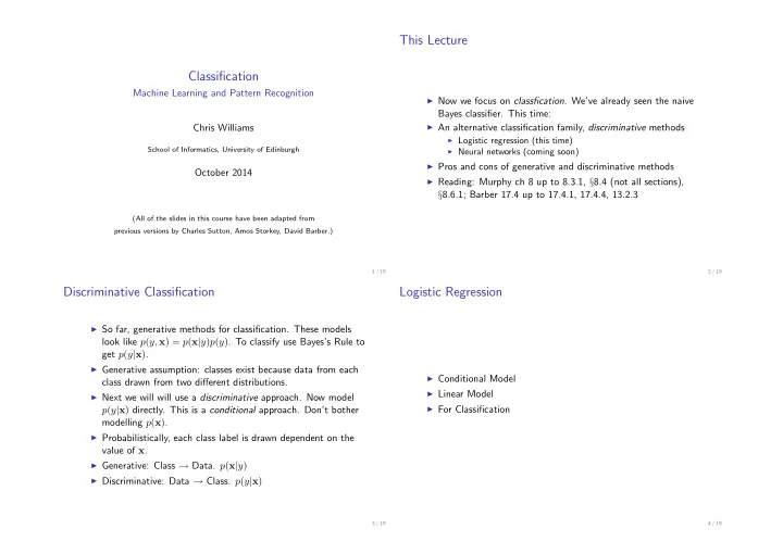
This Lecture Classification Machine Learning and Pattern Recognition ◮ Now we focus on classfication . We’ve already seen the naive Bayes classifier. This time: ◮ An alternative classification family, discriminative methods Chris Williams ◮ Logistic regression (this time) School of Informatics, University of Edinburgh ◮ Neural networks (coming soon) ◮ Pros and cons of generative and discriminative methods October 2014 ◮ Reading: Murphy ch 8 up to 8.3.1, § 8.4 (not all sections), § 8.6.1; Barber 17.4 up to 17.4.1, 17.4.4, 13.2.3 (All of the slides in this course have been adapted from previous versions by Charles Sutton, Amos Storkey, David Barber.) 1 / 19 2 / 19 Discriminative Classification Logistic Regression ◮ So far, generative methods for classification. These models look like p ( y, x ) = p ( x | y ) p ( y ) . To classify use Bayes’s Rule to get p ( y | x ) . ◮ Generative assumption: classes exist because data from each ◮ Conditional Model class drawn from two different distributions. ◮ Linear Model ◮ Next we will will use a discriminative approach. Now model ◮ For Classification p ( y | x ) directly. This is a conditional approach. Don’t bother modelling p ( x ) . ◮ Probabilistically, each class label is drawn dependent on the value of x . ◮ Generative: Class → Data. p ( x | y ) ◮ Discriminative: Data → Class. p ( y | x ) 3 / 19 4 / 19

Two Class Discrimination The logistic trick ◮ We need two things: ◮ Consider a two class case: y ∈ { 0 , 1 } . ◮ A function that returns probabilities (i.e. stays between 0 and 1 ). ◮ Use a model of the form ◮ But in regression (any form of regression) we used a function p ( y = 1 | x ) = g ( x ; w ) that returned values between ( −∞ and ∞ ). ◮ Use a simple trick to convert any regression model to a model ◮ g must be between 0 and 1 . Furthermore the fact that of class probabilities. Squash it! probabilities sum to one means ◮ The logistic (or sigmoid) function provides a means for this. p ( y = 0 | x ) = 1 − g ( x ; w ) ◮ g ( x ) = σ ( x ) ≡ 1 / (1 + exp( − x )) . ◮ As x goes from −∞ to ∞ , so σ ( x ) goes from 0 to 1 . ◮ What should we propose for g ? ◮ Other choices are available, but the logistic is the canonical link function 5 / 19 6 / 19 The Logistic Function That is it! Almost ◮ That is all we need. We can now convert any regression model to a classification model. 0.9 ◮ Consider linear regression f ( x ) = b + w T x . For linear 0.8 regression p ( y | x ) = N ( y ; f ( x ) , σ 2 ) is Gaussian with mean f . 0.7 ◮ Change the prediction by adding in the logistic function. This 0.6 changes the likelihood... 0.5 ◮ p ( y = 1 | x ) = σ ( f ( x )) = σ ( b + w T x ) . 0.4 0.3 ◮ Decision boundary p ( y = 1 | x ) = p ( y = 0 | x ) = 0 . 5 0.2 b + w T x = 0 0.1 −6 −4 −2 0 2 4 6 ◮ Linear regression/linear parameter models + logistic trick (use 1 The Logistic Function σ ( x ) = 1+exp( − x ) . of sigmoid squashing) = logistic regression. ◮ Probability of 1 changes with distance from some hyperplane. 7 / 19 8 / 19

The Linear Decision Boundary Logistic regression ◮ The bias parameter b shifts (for constant w ) the position of the hyperplane, but does not alter the angle. 0 ◮ The direction of the vector w affects the angle of the 0 0 0 0 hyperplane. The hyperplane is perpendicular to w . 0 w 1 1 0 ◮ The magnitude of the vector w effects how certain the 1 1 classifications are. 1 1 1 1 ◮ For small w most of the probabilities within a region of the decision boundary will be near to 0 . 5 . For two dimensional data the decision boundary is a line. ◮ For large w probabilities in the same region will be close to 1 or 0 . 9 / 19 10 / 19 Likelihood Gradients ◮ As before we can calculate the gradients of the log likelihood. ◮ Assume data is independent and identically distributed. ◮ Gradient of logistic function is σ ′ ( x ) = σ ( x )(1 − σ ( x )) . ◮ For parameters θ , the likelihood is p ( D| θ ) = N N p ( y = 1 | x n ) y n (1 − p ( y = 1 | x n )) 1 − y n � p ( y n | x n ) = � n =1 n =1 ◮ Hence the log likelihood is log p ( D| θ ) = N y n log p ( y = 1 | x n ) + (1 − y n ) log (1 − p ( y = 1 | x n )) � n =1 ◮ For maximum likelihood we wish to maximise this value w.r.t the parameters w and b . 11 / 19 12 / 19

Gradients 2D Example Prior w ∼ N (0 , 100 I ) ◮ As before we can calculate the gradients of the log likelihood. data Log−Likelihood 8 8 ◮ Gradient of logistic function is σ ′ ( x ) = σ ( x )(1 − σ ( x )) . 6 6 4 4 3 4 2 2 2 N 1 0 0 ( y n − σ ( b + w T x n )) x n � ∇ w L = (1) −2 −2 −4 −4 n =1 −6 −6 N ∂L −8 −8 −10 −5 0 5 −8 −6 −4 −2 0 2 4 6 8 ( y n − σ ( b + w T x n )) � ∂b = (2) Data MLE n =1 Log−Unnormalised Posterior 8 6 ◮ This cannot be solved directly to find the maximum. 4 ◮ Have to revert to an iterative procedure that searches for a 2 0 point where gradient is 0. −2 −4 ◮ This optimization problem is in fact convex. −6 −8 ◮ See later lecture. −8 −6 −4 −2 0 2 4 6 8 MAP Figure credit: Murphy Fig 8.5 12 / 19 13 / 19 Bayesian Logistic Regression 2D Example – Bayesian Prior w ∼ N (0 , 100 I ) p(y=1|x, wMAP) decision boundary for sampled w 8 8 6 6 4 4 ◮ Add a prior, e.g. w ∼ N (0 , V 0 ) 2 2 0 0 ◮ For linear regression integrals could be done analytically −2 −2 −4 −4 � −6 −6 p ( y ∗ | x ∗ , D ) = p ( y ∗ | x ∗ , w ) p ( w |D ) d w −8 −8 −8 −6 −4 −2 0 2 4 6 8 −10 −8 −6 −4 −2 0 2 4 6 8 samples from p ( w |D ) w MAP ◮ For logistic regression integrals are analytically intractable MC approx of p(y=1|x) 8 6 ◮ Use approximations, e.g. Gaussian approximation, Markov 4 chain Monte Carlo (see later) 2 0 −2 −4 −6 −8 −8 −6 −4 −2 0 2 4 6 8 Averaging over samples Figure credit: Murphy Fig 8.6 14 / 19 15 / 19

Multi-class targets Generalizing to features ◮ We can have categorical targets by using the softmax function on C target classes ◮ Rather than having one set of weights as in binary logistic regression, we have one set of weights for each class c ◮ Just as with regression, we can replace the x with features ◮ Have a separate set of weights w c , b c for each class c . Define φ ( x ) in logistic regression too. f c ( x ) = w ⊤ ◮ Just compute the features ahead of time. c x + b c ◮ Just as in regression, there is still the curse of dimensionality. ◮ Then exp( f c ( x )) p ( y = c | x ) = softmax ( f ( x )) = � c ′ exp( f c ′ ( x )) ◮ If C = 2 , this actually reduces to the logistic regression model we’ve already seen. 16 / 19 17 / 19 Generative and Discriminative Methods Summary ◮ Easier to fit? Naive Bayes is easy to fit, cf convex optimization problem for logistic regression ◮ Fit classes separately? In a discriminative model, all parameters interact ◮ The logistic function. ◮ Handle missing features easily? For generative models this ◮ Logistic regression. is easily handled (if features are missing at random) ◮ Hyperplane decision boundaries. ◮ Can handle unlabelled data? For generative models just ◮ The likelihood for logistic regression. model p ( x ) = � y p ( x | y ) p ( y ) ◮ Softmax for multi-class problems ◮ Symmetric in inputs and outputs? Discriminative methods ◮ Pros and cons of generative and discriminative methods model p ( y | x ) directly ◮ Can handle feature preprocessing? x → φ ( x ) . Big advantage of discriminative methods ◮ Well-calibrated probabilities? Some generative models (e.g. Naive Bayes) make strong assumptions, can lead to extreme probabilities 18 / 19 19 / 19