PRAM ALGORITHMS: POINTER JUMPING 2 1 08 08 2015 LIST RANKING - PDF document
08 08 2015 PARALLEL AND DISTRIBUTED ALGORITHMS BY DEBDEEP MUKHOPADHYAY AND ABHISHEK SOMANI http://cse.iitkgp.ac.in/~debdeep/courses_iitkgp/PAlgo/index.htm PRAM ALGORITHMS: POINTER JUMPING 2 1 08 08 2015 LIST RANKING
08 ‐ 08 ‐ 2015 PARALLEL AND DISTRIBUTED ALGORITHMS BY DEBDEEP MUKHOPADHYAY AND ABHISHEK SOMANI http://cse.iitkgp.ac.in/~debdeep/courses_iitkgp/PAlgo/index.htm PRAM ALGORITHMS: POINTER JUMPING 2 1
08 ‐ 08 ‐ 2015 LIST RANKING Consider the problem of finding, for each element of n elements on a linked list, the suffix sums of the last i elements of the list, where � � � � �. The suffix sum problem is a variant of the prefix sum problem. Array is replaced by a linked list. Sums are computed from the end. If the elements of the list are 0 or 1, and the associative operation is addition, the problem is called the list ranking problem. 3 LINK RANKING One way to solve this is to traverse the list and count the number of links traversed between the list element and the end of the list. Only a single pointer can be followed in one step, and there are n-1 pointers between the first element and the end of the list. How can any algorithm traverse such a list in less than Θ � time? 4 2
08 ‐ 08 ‐ 2015 PARALLELISATION We associate a processor with every list element and jump pointers in parallel! The distance to the end of the list is cut in half through the instruction : ���� � ← ��������� � � Hence, a logarithmic number of pointer jumpings are sufficient to collapse the list so that every element points to the last list element. If a processor adds to its own link traversal count, position[i], the current link traversal count of the successors it encounters, the list position will be correctly determined. 5 ILLUSTRATING THE PROCESS OF LIST RANKING List ranking problem Given a singly linked list L with n objects, for each node, compute the distance to the end of the list If d denotes the distance node.d = 0 if node.next = nil { node.next.d + 1 otherwise Serial algorithm: O(n) Parallel algorithm Assign one processor for each node Assume there are as many processors as list objects For each node i, perform 1. i.d = i.d + i.next.d 2. i.next = i.next.next // pointer jumping 3
08 ‐ 08 ‐ 2015 LIST RANKING – EXAMPLE 1 LIST RANKING – EXAMPLE 2 The position of each item on the n-element list can be determined in ���� �� pointer jumping steps. 8 4
08 ‐ 08 ‐ 2015 THE PRAM ALGORITHM Note this step does not depend on j. There are ���� �� steps. There are n processors. So total cost is: Θ�� log �� Not cost optimal! 9 THE SAME CODE USING POINTER NOTATIONS List_ranking(L) 1. for all P i for each node i, do 2. if i->next = null then i.d = 0 3. else i.d = 1 4. while(i->next != null) do 5. i.d = i.d + i->next.d 6. i->next = i->next->next 10 5
08 ‐ 08 ‐ 2015 LIST RANKING - DISCUSSIONS Synchronization is important In step 6 (i->next = i->next->next), all processors must read right hand side before any processor write left hand side The list ranking algorithm is EREW If we assume in step 5 (i.d = i.d + i.next.d) all processors read i.d and then read i.next.d If j.next = i, i and j do not read i.d concurrently Work performance performs O(n log n) work since n processors in O(log n) time Work efficient A PRAM algorithm is work efficient w.r.t another algorithm if two algorithms are within a constant factor Is the link ranking algorithm work-efficient w.r.t the serial algorithm? No, because O(n log n) versus O(n) Speedup S = n / log n PREORDER TREE TRAVERSAL Sometimes it is appropriate to reduce a complicated looking problem into a simpler form for which a parallel algorithm is already known. Let us consider the problem of numbering the vertices of a rooted tree in preorder (depth first search order). At first glance this problem looks sequential! 12 6
08 ‐ 08 ‐ 2015 RECURSIVE PREORDER TRAVERSAL Where is the parallelism? The fundamental operation PREORDER.TRAVERSAL(nodeptr): assigns a label to a node. Begin We cannot assign labels to the if nodeptr ≠ null then vertices in the right subtree of the left subtree, until we know nodecount nodecount + 1 how many vertices are on the nodeptr.label nodecount left subtree of the left subtree, and so on. PREORDER.TRAVERSAL(nodeptr.left) The algorithm seems inherently PREORDER.TRAVERSAL(nodeptr.right) sequential! endif Can we parallelize this? End 13 IDENTIFY THE CHARACTER 14 7
08 ‐ 08 ‐ 2015 IDENTIFY THE CHARACTER 15 IDENTIFY THE CHARACTER Robert Endre Tarjan (born April 30, 1948) is an American computer scientist and mathematician. He is the discoverer of several graph algorithms, including Tarjan's off-line least common ancestors algorithm, and co-inventor of both splay trees and Fibonacci heaps. Tarjan is currently the James S. McDonnell Distinguished University Professor of Computer Science at Princeton University, and the Chief Scientist at Intertrust Technologies (Source: Wiki) 16 8
08 ‐ 08 ‐ 2015 PARALLELIZATION OF THE TRAVERSAL Instead of focusing on the vertices, let us look into the edges. When we perform a preorder traversal, we systematically work our way through the edges of the tree. We pass along every vertex twice: one heading down from the parent to the child, and one going from the child to the parent. If we divide each tree edge into two edges, one corresponding to the downward traversal, and one corresponding to the upward traversal, then the problem of traversing a tree turns into the problem of traversing a single linked list. 17 TARJAN AND VISHKIN (1984) 4 steps: 1. The algorithm constructs a singly linked list. Each vertex of the linked list corresponds to a downward or upward edge traversal. 2. Algorithm assigns weights to the vertices of the newly created single linked list. For vertices corresponding to downward edges, the weight is 1 (it contributes to node count). For vertices corresponding to upward edges, the weight is 0 (it does not contribute to node count). 3. For each element of the singly-linked list, the rank of each element is determined (by pointer jumping). 4. The processors associated with the downward edges use the ranks they have computed to assign a preorder traversal number to their associated tree nodes (the tree node at the end of the downward edge). 18 9
08 ‐ 08 ‐ 2015 EXAMPLE a) Tree b) Double Tree Edges, distinguishing downward edges from upward edges. c) Build linked list out of directed tree edges. Associate 1 with downward edges, and 0 with upward edges. d) Use pointer jumping to compute total weight from each vertex to end of list. The elements of the linked list which correspond to downward edges, have been shaded. Processors managing these elements C,F assign preorder values. For example, (E,G) has a weight 4, meaning tree node G is 4 th node from end of preorder traversal list. The tree has 8 nodes, so it can compute that tree node G has label 5 in preorder traversal (=8-4+1) 19 DATA STRUCTURE FOR THE TREE For every tree node, the data structure stores the node’s parent, the node’s immediate sibling to the right, and the node’s leftmost child. Representing the node this way keeps the amount of data stored a constant for each tree node and simplifies the tree traversal. 20 10
08 ‐ 08 ‐ 2015 PROCESSOR ALLOCATION The PRAM algorithm spawns 2(n-1) processors. A tree with nodes have (n-1) edges. We are dividing each edge into two edges, one for the downward traversal and one for the upward traversal. So, the algorithm needs 2(n-1) processors to manipulate each of the 2(n-1) edges of the singly-linked list of elements corresponding to the edge traversals. 21 CONSTRUCTION OF THE LINKED LIST Once all the processors have been activated they construct the linked list: P(i,j): The processor for the edge (i,j) Note (j,i) has a different processor P(j,i) Given an edge (i,j), P(i,j) must compute the successor of (i,j) and store in a global array: succ[1…2(n-1)]. If the successor of (i,j) is (j,k), then succ[(i,j)] (j,k) 22 11
08 ‐ 08 ‐ 2015 HANDLING UPWARD EDGES Edge (i,j), such that parent(i)=j j If sibling[i] ≠ NULL succ[(i,j)] (j,sibling[i]) i k 23 HANDLING UPWARD EDGES Edge (i,j), such that parent(i)=j j If sibling[i] ≠ NULL succ[(i,j)] (j,sibling[i]) i k Else If parent[i] ≠ NULL k succ[(i,j)] (j,parent[i]) j i 24 12
08 ‐ 08 ‐ 2015 HANDLING UPWARD EDGES Edge (i,j), such that parent(i)=j j If sibling[i] ≠ NULL succ[(i,j)] (j,sibling[i]) i k Else If parent[i] ≠ NULL k succ[(i,j)] (j,parent[i]) Else succ[(i,j)] (i,j) j The edge is at the end of j the tree traversal, so we put a loop at the end of i i the element list. 25 HANDLING UPWARD EDGES Edge (i,j), such that parent(i)=j j If sibling[i] ≠ NULL succ[(i,j)] (j,sibling[i]) i k Else If parent[i] ≠ NULL k succ[(i,j)] (j,parent[i]) Else succ[(i,j)] (i,j) position[1…2(n-1)] j The edge is at the end of j is a global array to the tree traversal, so we j is the root. hold the edge ranks. put a loop at the end of position[j] 1 i i the element list. 26 13
08 ‐ 08 ‐ 2015 HANDLING DOWNWARD EDGES Edge (i,j), such that parent[i] ≠ j. i If child[j] ≠ NULL succ[(i,j)] (j,child[j]) i k 27 HANDLING DOWNWARD EDGES Edge (i,j), such that parent[i] ≠ j. i If child[j] ≠ NULL succ[(i,j)] (j,child[j]) i else succ[(i,j)] (j,i) k i ie. j is a leaf and the successor is the edge back from the child to the i parent. 28 14
Recommend
More recommend
Explore More Topics
Stay informed with curated content and fresh updates.
