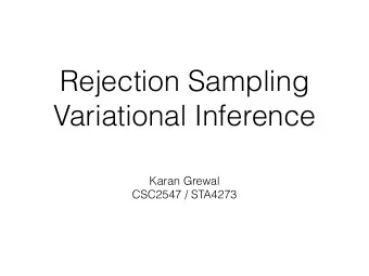
The Variational Predictive Natural Gradient Da Tang 1 Rajesh - PowerPoint PPT Presentation

The Variational Predictive Natural Gradient Da Tang 1 Rajesh Ranganath 2 1 Columbia University 2 New York University June 12, 2019

Variational Inference ◮ Latent variable models: p ( x , z ; θ ) = p ( z ) p ( x | z ; θ ).

Variational Inference ◮ Latent variable models: p ( x , z ; θ ) = p ( z ) p ( x | z ; θ ). ◮ Variational inference approximates the posterior through maximizing the ELBO : L ( λ , θ ) = E q [log p ( x | z ; θ )] − KL ( q ( z | x ; λ ) || p ( z )) .

Variational Inference ◮ Latent variable models: p ( x , z ; θ ) = p ( z ) p ( x | z ; θ ). ◮ Variational inference approximates the posterior through maximizing the ELBO : L ( λ , θ ) = E q [log p ( x | z ; θ )] − KL ( q ( z | x ; λ ) || p ( z )) . ∇ λ log q ( z | x ; λ ) · ∇ λ log q ( z | x ; λ ) ⊤ � ◮ q -Fisher Information F q = E q � (Hoffman et al., 2013) approximates the negative Hessian of the objective. λ L ( λ ) = F − 1 ◮ The natural gradient: ∇ NG · ∇ λ L ( λ ). q

-2.65e+10 100 -5.91e+09 75 VPNG Gradient -1.32e+09 50 -2.94e+08 25 -6.57e+07 0 -1.47e+07 −25 -3.27e+06 −50 Current -7.29e+05 Optimum -1.63e+05 −75 −75 −50 −25 0 25 50 75 100 125 150 Pathological Curvature of the ELBO ◮ The curvature of the ELBO may be pathological.

Pathological Curvature of the ELBO ◮ The curvature of the ELBO may be pathological. ◮ Example: A bivariate Gaussian model with unknown mean and known covariance � � 1 1 − ε Σ = , 0 < ε ≪ 1. 1 − ε 1 -2.65e+10 100 -5.91e+09 75 VPNG Gradient -1.32e+09 50 -2.94e+08 25 -6.57e+07 0 -1.47e+07 −25 -3.27e+06 −50 Current -7.29e+05 Optimum -1.63e+05 −75 −75 −50 −25 0 25 50 75 100 125 150

Pathological Curvature of the ELBO ◮ The curvature of the ELBO may be pathological. ◮ Example: A bivariate Gaussian model with unknown mean and known covariance � � 1 1 − ε Σ = , 0 < ε ≪ 1. 1 − ε 1 -2.65e+10 100 -5.91e+09 75 VPNG Gradient -1.32e+09 50 -2.94e+08 25 -6.57e+07 0 -1.47e+07 −25 -3.27e+06 −50 Current -7.29e+05 Optimum -1.63e+05 −75 −75 −50 −25 0 25 50 75 100 125 150 ◮ The natural gradient fails to help.

The Natural Gradient is Insufficient Limitations of the q -Fisher information: ◮ Approximates the Hessian of the objective well only when q ( z | x ; λ ) ≈ p ( z | x ; θ ). ◮ Ignore the model likelihood p ( x | z ; θ ) in computations.

The Variational Predictive Fisher Information ◮ Construct a positive definite matrix that resembles the negative Hessian of the expected log-likelihood part L ll = E q ( z | x ; λ ) [log p ( x | z ; θ )] of the ELBO .

The Variational Predictive Fisher Information ◮ Construct a positive definite matrix that resembles the negative Hessian of the expected log-likelihood part L ll = E q ( z | x ; λ ) [log p ( x | z ; θ )] of the ELBO . ◮ Reparameterize the variational distribution q : z = g ( x , ε ; λ ) ∼ q ( z | x ; λ ) ⇐ ⇒ ε ∼ s ( ε ) .

The Variational Predictive Fisher Information ◮ Construct a positive definite matrix that resembles the negative Hessian of the expected log-likelihood part L ll = E q ( z | x ; λ ) [log p ( x | z ; θ )] of the ELBO . ◮ Reparameterize the variational distribution q : z = g ( x , ε ; λ ) ∼ q ( z | x ; λ ) ⇐ ⇒ ε ∼ s ( ε ) . ◮ The variational predictive Fisher information: F r = E ε [ E p ( x ′ | z = g ( x , ε ; λ ); θ ) [ ∇ λ , θ log p ( x ′ | z = g ( x , ε ; λ ); θ ) · ∇ λ , θ log p ( x ′ | z = g ( x , ε ; λ ); θ ) ⊤ ]] , exactly the “expected” Fisher information of the reparameterized predictive distribution p ( x ′ | z = g ( x , ε ; λ ); θ ).

The Variational Predictive Fisher Information ◮ Variational predictive Fisher captures the curvature of variational inference.

The Variational Predictive Fisher Information ◮ Variational predictive Fisher captures the curvature of variational inference. ◮ Matrix spectrum comparison (for the bivariate Gaussian example): (d) Precision mat Σ − 1 (e) q -Fisher info F q (f) Our Fisher info F r

The Variational Predictive Natural Gradient ◮ The variational predictive natural gradient (VPNG): ∇ VPNG L = F − 1 · ∇ λ , θ L ( λ , θ ) . λ , θ r

The Variational Predictive Natural Gradient ◮ The variational predictive natural gradient (VPNG): ∇ VPNG L = F − 1 · ∇ λ , θ L ( λ , θ ) . λ , θ r ◮ In practice, use Monte Carlo estimations to approximate F r and add a small dampening parameter to ensure invertibility.

Experiments: Bayesian Logistic Regression ◮ Tested on synthetic data with high correlations. ◮ Empirical results: Method Train AUC Test AUC Gradient 0 . 734 ± 0 . 017 0 . 718 ± 0 . 022 NG 0 . 744 ± 0 . 043 0 . 751 ± 0 . 047 VPNG 0 . 972 ± 0 . 011 0 . 967 ± 0 . 011 Table: Bayesian Logistic regression AUC

Experiments: VAE and VMF 80 100 100 Train ELBO Test ELBO 120 120 140 140 Gradient Gradient NG NG 160 160 VPNG VPNG 180 0 200 400 600 800 1000 0 200 400 600 800 1000 Time (s) Time (s) −700 −800 −800 −900 Train ELBO −900 Test ELBO −1000 −1000 Gradient Gradient −1100 −1100 NG NG −1200 −1200 VPNG VPNG 500 1000 1500 2000 2500 3000 500 1000 1500 2000 2500 3000 Time (s) Time (s) Figure: Learning curves of variational autoencoders (upper) and variational matrix factorization (lower) on real datasets.

Conclusion and Future Work ◮ The VPNG corrects for curvature in the objective between the parameters in variational inference.

Conclusion and Future Work ◮ The VPNG corrects for curvature in the objective between the parameters in variational inference. ◮ Future work includes extending to general Bayesian networks with multiple stochastic layers.

Thanks! Poster #234 Code available at https://github.com/datang1992/VPNG.