The story of the film so far... X a c.r.v. with p.d.f. f and g : R R - PowerPoint PPT Presentation

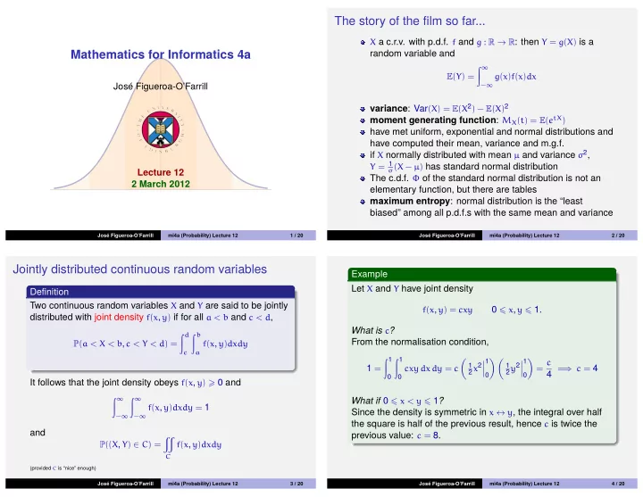
The story of the film so far... X a c.r.v. with p.d.f. f and g : R → R : then Y = g ( X ) is a Mathematics for Informatics 4a random variable and � ∞ E ( Y ) = g ( x ) f ( x ) dx Jos´ e Figueroa-O’Farrill − ∞ variance : Var ( X ) = E ( X 2 ) − E ( X ) 2 moment generating function : M X ( t ) = E ( e tX ) have met uniform, exponential and normal distributions and have computed their mean, variance and m.g.f. if X normally distributed with mean µ and variance σ 2 , Y = 1 σ ( X − µ ) has standard normal distribution Lecture 12 The c.d.f. Φ of the standard normal distribution is not an 2 March 2012 elementary function, but there are tables maximum entropy : normal distribution is the “least biased” among all p.d.f.s with the same mean and variance Jos´ e Figueroa-O’Farrill mi4a (Probability) Lecture 12 1 / 20 Jos´ e Figueroa-O’Farrill mi4a (Probability) Lecture 12 2 / 20 Jointly distributed continuous random variables Example Let X and Y have joint density Definition Two continuous random variables X and Y are said to be jointly f ( x , y ) = cxy 0 � x , y � 1. distributed with joint density f ( x , y ) if for all a < b and c < d , What is c ? � d � b From the normalisation condition, P ( a < X < b , c < Y < d ) = f ( x , y ) dxdy c a � 1 � 1 � 1 � � 1 � = c 2 x 2 � 2 y 2 � 1 1 1 = ⇒ c = 4 cxy dx dy = c � � 4 = � � 0 0 0 0 It follows that the joint density obeys f ( x , y ) � 0 and � ∞ � ∞ What if 0 � x < y � 1 ? f ( x , y ) dxdy = 1 Since the density is symmetric in x ↔ y , the integral over half − ∞ − ∞ the square is half of the previous result, hence c is twice the and previous value: c = 8. � P (( X , Y ) ∈ C ) = f ( x , y ) dxdy C (provided C is “nice” enough) Jos´ e Figueroa-O’Farrill mi4a (Probability) Lecture 12 3 / 20 Jos´ e Figueroa-O’Farrill mi4a (Probability) Lecture 12 4 / 20

Uniform joint densities Marginals Let A ⊂ R 2 be a region with area | A | . Definition Let X , Y be continuous random variables with joint density X and Y are (jointly) uniform in A if f ( x , y ) . Then the marginal p.d.f.s f X ( x ) and f Y ( y ) are given by � 1 � ∞ � ∞ | A | , ( x , y ) ∈ A f X ( x ) = f ( x , y ) dy and f Y ( y ) = f ( x , y ) dx f ( x , y ) = − ∞ − ∞ 0, elsewhere Remark Example As in the discrete case there is no need to stop at two random Let X , Y be jointly uniform in the unit disk variables, and we can have joint densities f ( x 1 , . . . , x n ) for n D = { ( x , y ) | x 2 + y 2 � 1 } . Then | D | = π , whence jointly distributed random variables, with many different marginals. f ( x , y ) = 1 0 � x 2 + y 2 � 1 π Jos´ e Figueroa-O’Farrill mi4a (Probability) Lecture 12 5 / 20 Jos´ e Figueroa-O’Farrill mi4a (Probability) Lecture 12 6 / 20 Joint distributions Example Let X , Y be jointly uniform on the unit disk D : Definition Let X and Y be continuous random variables with joint density f ( x , y ) = 1 0 � x 2 + y 2 � 1 f ( x , y ) . Their joint distribution is defined as π � x � y The marginals are given by F ( x , y ) = P ( X � x , Y � y ) = f ( u , v ) du dv − ∞ − ∞ � √ 1 − x 2 1 πdy = 2 y � 1 − x 2 f X ( x ) = � 1 − x 2 − √ π 1 − x 2 It follows from the fundamental theorem of calculus that for − 1 � x � 1 and, by symmetry, ∂ 2 x f ( x , y ) = ∂x∂yF ( x , y ) f Y ( y ) = 2 � 1 − y 2 � 1 − x 2 − π and the marginal distributions are obtained by for − 1 � y � 1 F X ( x ) = F ( x , ∞ ) and F Y ( y ) = F ( ∞ , y ) Jos´ e Figueroa-O’Farrill mi4a (Probability) Lecture 12 7 / 20 Jos´ e Figueroa-O’Farrill mi4a (Probability) Lecture 12 8 / 20

Independence Example Let X , Y be jointly distributed with f ( x , y ) = x + y on 0 � x , y � 1. Definition � 1 � 1 One checks that indeed 0 ( x + y ) dxdy = 1. Two continuous random variables X and Y are independent if 0 The joint distribution is F ( x , y ) = F X ( x ) F Y ( y ) � x � y F ( x , y ) = ( u + v ) du dv 0 0 or, equivalently, � x � � y � f ( x , y ) = f X ( x ) f Y ( y ) . = ( u + v ) dv du 0 0 � x � 2 y 2 � uy + 1 = du It follows that for X , Y independent 0 = 1 2 x 2 y + 1 2 xy 2 for 0 � x , y � 1 P ( X ∈ A , Y ∈ B ) = P ( X ∈ A ) P ( Y ∈ B ) For y > 1, F ( x , y ) = 1 2 x ( x + 1 ) and similarly, for x > 1, F ( x , y ) = 1 2 y ( y + 1 ) . Useful criterion : X and Y are independent iff f ( x , y ) = g ( x ) h ( y ) . � Then f X ( x ) = cg ( x ) and f Y ( y ) = 1 c h ( y ) , where c = R h ( y ) dy . Jos´ e Figueroa-O’Farrill mi4a (Probability) Lecture 12 9 / 20 Jos´ e Figueroa-O’Farrill mi4a (Probability) Lecture 12 10 / 20 Geometric probability Examples X and Y are jointly uniform on 0 � x � a and 0 � y � b : Geometric probability or “continuous combinatorics” 1 studies geometric objects sharing a common probability f ( x , y ) = 1 space. for ( x , y ) ∈ [ 0, a ] × [ 0, b ] ab We have already seen some geometric probability with marginals f X ( x ) = 1 a and f Y ( y ) = 1 problems in the tutorial sheets. b . Since f ( x , y ) = f X ( x ) f Y ( y ) , X and Y are independent. For example, in Tutorial Sheet 4 you considered the X and Y are jointly uniform on the disk 0 � x 2 + y 2 � a 2 : problem of tossing a coin on a square grid and computing 2 the probability that the coin is fully contained inside one of 1 for 0 � x 2 + y 2 � a 2 the squares. f ( x , y ) = πa 2 This game was called franc-carreau (“free tile”) in France and was studied by Buffon in his treatise Sur le jeu de � a 2 − x 2 and 1 with marginals f X ( x ) = πa 2 franc-carreau (1733). a 2 − y 2 . Since f ( x , y ) � = f X ( x ) f Y ( y ) , X and Y 1 � f Y ( y ) = πa 2 In probability, Buffon is perhaps better known for Buffon’s are not independent. needle , which is a paradigmatic geometric probability problem. Jos´ e Figueroa-O’Farrill mi4a (Probability) Lecture 12 11 / 20 Jos´ e Figueroa-O’Farrill mi4a (Probability) Lecture 12 12 / 20

Buffon’s needle I Buffon’s needle II The needle is described by the Drop a needle of length ℓ at midpoint and the angle with the random on a striped floor, with horizontal. stripes a distance L apart. x θ Symmetry allows us to ignore the Let ℓ < L : short needles. vertical component of the midpoint and to assume the horizontal component lies in one of the strips. L Let X denote the horizontal component of the midpoint. It is uniformly distributed in [− L 2 , L 2 ] . ℓ Let Θ denote the angle with the horizontal, which is uniformly distributed in [− π 2 , π 2 ] . Since X and Θ are independent, the joint probability density function is the product of the two probability density functions and hence is also uniformly distributed. What is the probability that the needle does not touch any line? Jos´ e Figueroa-O’Farrill mi4a (Probability) Lecture 12 13 / 20 Jos´ e Figueroa-O’Farrill mi4a (Probability) Lecture 12 14 / 20 Buffon’s needle III Functions of several random variables The needle will touch one of the parallel lines if and only if X and Y are continuous random variables with joint density | x | + ℓ 2 cos θ > L x θ f ( x , y ) 2 Z = g ( X , Y ) , for some function g : R 2 → R for x ∈ [− L 2 , L 2 ] and θ ∈ [− π 2 , π 2 ] . How is Z distributed? (assuming it is a c.r.v.) The complementary probability is Its c.d.f. F Z ( z ) = P ( Z � z ) is given by � π � � 1 � 2 ( L − ℓ cos θ ) = 1 2 � � | X | � 1 2 ( L − ℓ cos Θ ) � P dx dθ F Z ( z ) = f ( x , y ) dx dy Lπ − π − 1 2 ( L − ℓ cos θ ) 2 g ( x , y ) � z � π = 1 2 ( L − ℓ cos θ ) dθ Lπ − π Its p.d.f. f Z ( z ) = F ′ 2 Z ( z ) � π cos θdθ = 1 − 2 ℓ = 1 − ℓ 2 Lπ Lπ − π 2 Jos´ e Figueroa-O’Farrill mi4a (Probability) Lecture 12 15 / 20 Jos´ e Figueroa-O’Farrill mi4a (Probability) Lecture 12 16 / 20