The story of the film so far... (Temporally homogeneous) Markov - PowerPoint PPT Presentation

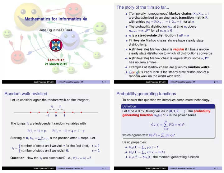
The story of the film so far... (Temporally homogeneous) Markov chains { X 0 , X 1 , . . . } are characterised by an stochastic transition matrix P , Mathematics for Informatics 4a with entries p ij = P ( X n + 1 = j | X n = i ) for all n The probability distribution π m at time m obeys π m + n = π m P n for all m , n � 0 José Figueroa-O’Farrill π is a steady-state distribution if πP = π Finite-state Markov chains always have steady state distributions. A (finite-state) Markov chain is regular if it has a unique steady state distribution to which all distributions converge A (finite-state) Markov chain is regular iff for some n , P n Lecture 17 has no zero entries. 21 March 2012 Examples of Markov chains are given by random walks ’s PageRank is the steady-state distribution of a random walk on the world wide web. José Figueroa-O’Farrill mi4a (Probability) Lecture 17 1 / 1 José Figueroa-O’Farrill mi4a (Probability) Lecture 17 2 / 1 Random walk revisited Probability generating functions Let us consider again the random walk on the integers: To answer this question we introduce some more technology. q p Definition Let X be a d.r.v. taking values in { 0, 1, 2, . . . } . The probability generating function G X ( s ) of X is the power series − 1 0 1 ∞ � The jumps J i are independent random variables with P ( X = n ) s n G X ( s ) = n = 0 P ( J i = 1 ) = p P ( J i = − 1 ) = q = 1 − p which agrees with E ( s X ) = � x p ( x ) s x . Starting at 0, X n = � n i = 1 J i is the position after n steps. Let Basic properties: � number of steps until we visit r for the first time, r � = 0 G X ( 1 ) = � x p ( x ) = 1 T r = number of steps until we revisit 0, r = 0. X ( 1 ) = � G ′ x xp ( x ) = E ( X ) G X ( e t ) = M X ( t ) , the moment generating function Question : How the T r are distributed? i.e., P ( T r = n ) = ? José Figueroa-O’Farrill mi4a (Probability) Lecture 17 3 / 1 José Figueroa-O’Farrill mi4a (Probability) Lecture 17 4 / 1

Behaviour under independence Examples Theorem Let X be binomial with parameters ( n , p ) , so 1 Let X , Y be independent d.r.v.s with probability generating � n � p r q n − r , for 0 � r � n and with q = 1 − p . Then p ( r ) = r functions G X ( s ) and G Y ( s ) . Then n n � � � n � p ( r ) s r = p r q n − r s r = ( q + ps ) n G X ( s ) = G X + Y ( s ) = G X ( s ) G Y ( s ) r r = 0 r = 0 using the binomial theorem. Proof is mutatis mutandis as for moment generating functions. Let X be geometrically distributed with parameter p , so that 2 p ( k ) = q k − 1 p for k � 1 and again q = 1 − p . Then Example Let X = � n k = 1 I k , where I k are independent Bernoulli trials with ∞ ∞ ∞ � � � ps p ( k ) s k = q k − 1 ps k = ps ( qs ) n = 1 − qs , G X ( s ) = success probability p . Then G I k ( s ) = q + ps , with q = 1 − p , and k = 1 k = 1 n = 0 n n � � ( q + ps ) = ( q + ps ) n , G X ( s ) = G I k ( s ) = for | s | < 1 q . k = 1 k = 1 The P ( X = n ) are obtained by expanding G X ( s ) in powers of s . whence X is binomial with parameters ( n , p ) , as expected. José Figueroa-O’Farrill mi4a (Probability) Lecture 17 5 / 1 José Figueroa-O’Farrill mi4a (Probability) Lecture 17 6 / 1 Conditional expectation I Conditional expectation II Interchanging the order of the sums, Definition � � � Let X , Y be random variables with joint distribution p X , Y ( x , y ) . E ( X ) = xp ( x | y ) p Y ( y ) = E ( X | Y = y ) p Y ( y ) Then the conditional distribution of X given Y is y x y which defines the conditional expectation of X given Y : p ( x | y ) = P ( X = x | Y = y ) = P ( { X = x } ∩ { Y = y } ) = p X , Y ( x , y ) P ( { Y = y } ) p Y ( y ) � E ( X | Y = y ) = xp ( x | y ) x It follows that the marginal distribution This defines a random variable E ( X | Y ) , which is a function of Y , whose value at y is E ( X | Y = y ) . Thus we have � � p X , Y ( x , y ) = p X ( x ) = p ( x | y ) p Y ( y ) E ( X ) = E ( E ( X | Y )) y y so that and similarly for any function Z = h ( X ) , � � � E ( X ) = xp X ( x ) = xp ( x | y ) p Y ( y ) � where E ( Z ) = E ( E ( Z | Y )) E ( Z | Y = y ) = h ( x ) p ( x | y ) x x y x José Figueroa-O’Farrill mi4a (Probability) Lecture 17 7 / 1 José Figueroa-O’Farrill mi4a (Probability) Lecture 17 8 / 1

Example (Gambler’s ruin – revisited) Example (Random sums) A gambler starts with £ k and makes a number of independent Let X 1 , X 2 , . . . be i.i.d. and let N be an N -valued d.r.v. independent from the X i . Let T = � N £1 bets with even odds. The gambler stops when she has either r = 0 X r . What is G T ( s ) ? £0 or £ N . Let T k be the length of the game. What is E ( T k ) ? We calculate this by conditioning on N : Conditioning on the result of the first bet, and letting τ k = E ( T k ) , � E ( s T | N = n ) P ( N = n ) E ( s T ) = τ k = E ( T k | win ) P ( win ) + E ( T k | lose ) P ( lose ) n = 1 2 ( 1 + τ k + 1 ) + 1 2 ( 1 + τ k − 1 ) By independence, = 1 + 1 for 0 < k < n 2 ( τ k + 1 + τ k − 1 ) E ( s T | N = n ) = E ( s X 1 + ··· + X n ) = E ( s X 1 ) . . . E ( s X n ) = ( G X ( s )) n whereas τ 0 = τ N = 0. τ k is quadratic in k with zeroes at 0 and where G X ( s ) is the p.g.f. of any of the X i . Hence N , so τ k = ck ( N − k ) for some constant c . Plugging it into the equation for k = 1, we see that c = 1 and hence � G X ( s ) n P ( N = n ) = E ( G X ( s ) N ) = G N ( G X ( s )) G T ( s ) = n E ( T k ) = k ( N − k ) In particular, E ( T ) = G ′ T ( 1 ) = G ′ N ( G X ( 1 )) G ′ X ( 1 ) = E ( N ) E ( X ) José Figueroa-O’Farrill mi4a (Probability) Lecture 17 9 / 1 José Figueroa-O’Farrill mi4a (Probability) Lecture 17 10 / 1 The Galton–Watson problem I The Galton–Watson problem II In 1873, Francis Galton posed a problem The problem was (partially) solved by the out of his concern in the decay of families Reverend Henry Watson, a of “men of note”. In more modern mathematician, who together with Galton language, a similar problem is the wrote On the probability of extinction of following. families in 1874. It gave rise to a class of A population of individuals reproduces problems known as branching itself in generations. Let X n denote the processes . size of the population in the n th generation. There are two rules: • • each member of a generation produces a family (maybe of 1 • size 0) in the next generation • • • family sizes of all individuals are i.i.d. random variables 2 • • If we assume that X 0 = 1 , what is the probability that X n = 0 for some n ? i.e., will the family become extinct? • • José Figueroa-O’Farrill mi4a (Probability) Lecture 17 11 / 1 José Figueroa-O’Farrill mi4a (Probability) Lecture 17 12 / 1

The Galton–Watson problem III The Galton–Watson problem IV We are interested in the large n limit, call it z . If z exists, it obeys The population at the n th generation is a random sum of G ( z ) = z . Formally, if G n ( 0 ) → z as n → ∞ , applying G again to random variables: X n − 1 both sides, we have G n + 1 ( 0 ) → G ( z ) , but G n + 1 ( 0 ) → z , hence � ξ ( n − 1 ) X n = G ( z ) = z . We can also see this graphically: j j = 1 0.7 where ξ ( n − 1 ) is the size of the family of the j th individual of the 0.6 j ( n − 1)st generation. They are i.i.d. with p.g.f. G ( s ) . Let us write 0.5 random sums example , G n ( s ) for the p.g.f. of X n . Then by the 0.4 0.3 G n ( s ) = G n − 1 ( G ( s )) = G n − 2 ( G ( G ( s ))) = · · · = G n ( s ) 0.2 0.1 i.e., the n th iterate of G . 0.1 0.2 0.3 0.4 0.5 0.6 0.7 There is always one solution: z = 1, namely extinction ! G n is the p.g.f. of X n , whence Watson concluded (incorrectly) that extinction was ∞ � inevitable. P ( X n = j ) s j ⇒ P ( X n = 0 ) = G n ( 0 ) = G n ( 0 ) G n ( s ) = = Luckily (?) that’s not always the case. j = 0 José Figueroa-O’Farrill mi4a (Probability) Lecture 17 13 / 1 José Figueroa-O’Farrill mi4a (Probability) Lecture 17 14 / 1 Example (Extinction and survival for Poisson branching) Example (Extinction and survival for “geometric” branching) Suppose that the family sizes are Poisson distributed, so that Suppose that the family sizes are distributed by a geometric distribution p ( k ) = q k p for k � 0 and q = 1 − p . Then ∞ � k ! s k = e − λ e λs = e λ ( s − 1 ) e − λ λ k G ( s ) = ∞ � p q k ps k = G ( s ) = k = 0 1 − qs k = 0 We must solve the equation e λ ( z − 1 ) = z for 0 � z � 1. For λ � 1 p We must solve the equation 1 − qz = z for 0 � z � 1. It has two the only solution is z = 1, so the family will be extinct with roots (for q � = 0, otherwise z = 1) probability 1, but for λ > 1 there is a nonzero probability of survival: � � ( 2 p − 1 ) 2 z = 1 ± 1 − 4 pq = 1 ± 1.0 1.0 2 q 2 ( 1 − p ) 0.8 0.8 p so one root is always 1 (extinction) and the other is 1 − p , which 0.6 0.6 is < 1 only for p < 1 2 . So if p � 1 2 , extinction is inevitable, but if 0.4 0.4 p < 1 2 there is a chance of survival. 0.2 0.2 0.2 0.4 0.6 0.8 1.0 0.2 0.4 0.6 0.8 1.0 José Figueroa-O’Farrill mi4a (Probability) Lecture 17 15 / 1 José Figueroa-O’Farrill mi4a (Probability) Lecture 17 16 / 1