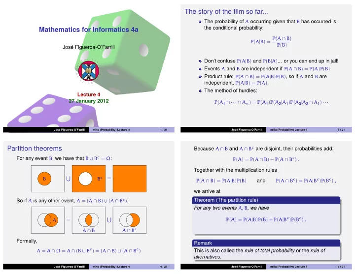
The story of the film so far... The probability of A occurring given - PowerPoint PPT Presentation

The story of the film so far... The probability of A occurring given that B has occurred is the conditional probability: Mathematics for Informatics 4a P ( A | B ) = P ( A ∩ B ) P ( B ) Jos´ e Figueroa-O’Farrill Don’t confuse P ( A | B ) and P ( B | A ) ... or you can end up in jail! Events A and B are independent if P ( A ∩ B ) = P ( A ) P ( B ) Product rule: P ( A ∩ B ) = P ( A | B ) P ( B ) , so if A and B are independent, P ( A | B ) = P ( A ) . The method of hurdles: Lecture 4 27 January 2012 P ( A 1 ∩ · · · ∩ A n ) = P ( A 1 ) P ( A 2 | A 1 ) P ( A 3 | A 2 ∩ A 1 ) · · · Jos´ e Figueroa-O’Farrill mi4a (Probability) Lecture 4 1 / 21 Jos´ e Figueroa-O’Farrill mi4a (Probability) Lecture 4 3 / 21 Because A ∩ B and A ∩ B c are disjoint, their probabilities add: Partition theorems For any event B , we have that B ∪ B c = Ω : P ( A ) = P ( A ∩ B ) + P ( A ∩ B c ) . Together with the multiplication rules � = B c B P ( A ∩ B c ) = P ( A | B c ) P ( B c ) , P ( A ∩ B ) = P ( A | B ) P ( B ) and we arrive at So if A is any other event, A = ( A ∩ B ) ∪ ( A ∩ B c ) : Theorem (The partition rule) For any two events A , B , we have P ( A ) = P ( A | B ) P ( B ) + P ( A | B c ) P ( B c ) . = � A A ∩ B c A ∩ B Formally, Remark A = A ∩ Ω = A ∩ ( B ∪ B c ) = ( A ∩ B ) ∪ ( A ∩ B c ) This is also called the rule of total probability or the rule of alternatives . Jos´ e Figueroa-O’Farrill mi4a (Probability) Lecture 4 4 / 21 Jos´ e Figueroa-O’Farrill mi4a (Probability) Lecture 4 5 / 21

A geometric analogy A general partition rule Consider R 2 with the standard dot product: Definition By a (finite) partition of Ω we mean events { B 1 , B 2 , . . . , B n } x · y = ( x 1 , x 2 ) · ( y 1 , y 2 ) = x 1 y 1 + x 2 y 2 . such that B i ∩ B j = ∅ for i � = j and � n i = 1 B i = Ω . Let ( e 1 , e 2 ) be an orthonormal basis for R 2 : Theorem (General partition rule) e 2 � 1 i = j Let { B 1 , . . . , B n } be a partition of Ω . Then for any event A , e i · e j = 0 i � = j n e 1 � P ( A | B i ) P ( B i ) . P ( A ) = Any vector x ∈ R 2 can be decomposed in an unique way as i = 1 x = ( x · e 1 ) e 1 + ( x · e 2 ) e 2 P ( A ) = P ( A | B ) P ( B ) + P ( A | B c ) P ( B c ) cf. Proof. This is proved in exactly the same way as in the case of the The analogue of orthogonality is now P ( B | B c ) = 0. partition { B , B c } . Jos´ e Figueroa-O’Farrill mi4a (Probability) Lecture 4 6 / 21 Jos´ e Figueroa-O’Farrill mi4a (Probability) Lecture 4 7 / 21 Example (More coins) Example (Medical tests) A box contains 3 double-headed coins, 2 double-tailed coins A virus infects a proportion p of individuals in a given and 5 conventional coins. You pick a coin at random and flip it. population. A test is devised to indicate whether a given What is the probability that you get a head? individual is infected. The probability that the test is positive for Let H be the event that you get a head and let A , B , C be the an infected individual is 95%, but there is a 10% probability of a events that the coin you picked was double-headed, false positive. Testing an individual at random, what is the double-tailed or conventional, respectively. chance of a positive result? Then by the (general) partition rule Let P denote the event that the result of the test is positive and V the event that the individual is infected. Then P ( H ) = P ( H | A ) P ( A ) + P ( H | B ) P ( B ) + P ( H | C ) P ( C ) P ( P ) = P ( P | V ) P ( V ) + P ( P | V c ) P ( V c ) = ( 1 × 3 10 ) + ( 0 × 2 10 ) + ( 1 2 × 5 10 ) = 0.95 p + 0.1 ( 1 − p ) = 3 10 + 1 4 = 11 20 = 0.85 p + 0.1 (Not a very good test: if p is very small, most positive results are false positives.) Jos´ e Figueroa-O’Farrill mi4a (Probability) Lecture 4 8 / 21 Jos´ e Figueroa-O’Farrill mi4a (Probability) Lecture 4 9 / 21

Conditional partition rule Example (Noisy channels) Alice and Bob communicate across a noisy channel using a bit Theorem stream. Let S 0 (resp. S 1 ) denote the event that a 0 (resp. 1 ) was Let { B 1 , . . . , B n } be a partition of Ω and let C be an event with sent, and let R 0 (resp. R 1 ) denote the event that a 0 (resp. 1 ) P ( C ) > 0 . Then for any event A , was received. Suppose that P ( S 0 ) = 4 7 and that due to the noise n P ( R 1 | S 0 ) = 1 8 and P ( R 0 | S 1 ) = 1 6 . What is P ( S 0 | R 0 ) ? � P ( A | B i ∩ C ) P ( B i | C ) . P ( A | C ) = P ( S 0 | R 0 ) = P ( S 0 ∩ R 0 ) P ( S 0 ∩ R 0 ) i = 1 = P ( R 0 ) P ( S 0 ∩ R 0 ) + P ( S 1 ∩ R 0 ) Proof P ( S 1 ∩ R 0 ) = P ( R 0 | S 1 ) P ( S 1 ) = P ( R 0 | S 1 )( 1 − P ( S 0 )) = 1 6 × 3 7 = 1 The partition rule holds in any probability space, so in particular 14 it holds for the conditional probability P ′ ( A ∩ C ) = P ( A | C ) . Since P ( S 0 ∩ R 0 ) = P ( R 0 | S 0 ) P ( S 0 ) = ( 1 − P ( R 1 | S 0 )) P ( S 0 ) = 7 8 × 4 7 = 1 2 { B 1 ∩ C , . . . , B n ∩ C } is a partition of C , n � � P ( S 0 | R 0 ) = 1 ( 1 2 + 1 14 ) = 1 7 = 7 4 � P ′ ( A ∩ C ) = P ′ ( A ∩ C | B i ∩ C ) P ′ ( B i ∩ C ) ∴ 2 2 8 i = 1 Jos´ e Figueroa-O’Farrill mi4a (Probability) Lecture 4 10 / 21 Jos´ e Figueroa-O’Farrill mi4a (Probability) Lecture 4 11 / 21 Example Proof (continued) We rewrite P ′ ( A ∩ C ) = � n There are number of different drugs to treat a disease and each i = 1 P ′ ( A ∩ C | B i ∩ C ) P ′ ( B i ∩ C ) as drug may give rise to side effects. A certain drug C has a 99% n success rate in the absence of side effects and side effects only � P ′ ( A ∩ C | B i ∩ C ) P ( B i | C ) . P ( A | C ) = arise in 5% of cases. If they do arise, however, then C has only i = 1 a 30% success rate. If C is used, what is the probability of the event A that a cure is effected? We finish the proof by rewriting P ′ ( A ∩ C | B i ∩ C ) as follows Let B be the event that no side effects occur. We are given that P ′ ( A ∩ C | B i ∩ C ) = P ′ ( A ∩ B i ∩ C ) = P ( A ∩ B i | C ) P ( A | B c ∩ C ) = 0.3 , P ′ ( B i ∩ C ) P ( B i | C ) P ( A | B ∩ C ) = 0.99 P ( B | C ) = 0.95 = P ( A ∩ B i ∩ C ) � P ( B i ∩ C ) whence P ( B c | C ) = 0.05. By the conditional partition rule P ( C ) P ( C ) corresponding to the partition { B , B c } and condition C , = P ( A ∩ B i ∩ C ) P ( B i ∩ C ) P ( A | C ) = P ( A | B ∩ C ) P ( B | C ) + P ( A | B c ∩ C ) P ( B c | C ) = P ( A | B i ∩ C ) . = ( 0.99 × 0.95 ) + ( 0.3 × 0.05 ) = 0.9555 ≃ 96% Jos´ e Figueroa-O’Farrill mi4a (Probability) Lecture 4 12 / 21 Jos´ e Figueroa-O’Farrill mi4a (Probability) Lecture 4 13 / 21

Bayes’s rule Example (False positives) Recall the product rule the earlier example and it shows You get tested for the virus in positive. What is the probability that you are actually infected? P ( A ∩ B ) = P ( A | B ) P ( B ) = P ( B | A ) P ( A ) , the earlier example , we want to compute P ( V | P ) . By In the notation of Bayes’s rule which immediately gives Theorem (Bayes’s rule) P ( V | P ) = P ( P | V ) P ( V ) 0.95 p = 0.85 p + 0.1 P ( P ) P ( A | B ) = P ( B | A ) P ( A ) P ( B ) So that if half the population is infected ( p = 0.5), then P ( V | P ) ≃ 90% and the test looks good, but if the virus affects only one person in every thousand ( p = 10 − 3 ), then Using the partition rule P ( B ) = P ( B | A ) P ( A ) + P ( B | A c ) P ( A c ) we P ( V | P ) ≃ 1%, so not very conclusive at all! get a modified version of Bayes’s rule: Theorem (Bayes’s rule too) P ( B | A ) P ( A ) P ( A | B ) = P ( B | A ) P ( A ) + P ( B | A c ) P ( A c ) Jos´ e Figueroa-O’Farrill mi4a (Probability) Lecture 4 14 / 21 Jos´ e Figueroa-O’Farrill mi4a (Probability) Lecture 4 15 / 21 Example (Multiple choice exam) Example (Multiple choice exam – continued) A student is taking a multiple choice exam, each question We notice that P ( A | K ) = 1 and P ( A | K c ) = 1 /c , whence having c available choices. The student either knows the P ( A ) = P ( A | K ) P ( K ) + P ( A | K c ) P ( K c ) answer to the question with probability p or else guesses at random with probability 1 − p . Given that the answer selected is = ( 1 × p ) + ( 1 c × ( 1 − p )) correct, what is the probability that the student knew the = p + 1 − p . answer? c Let A denote the event that the answer is correct and let K Finally, denote the event that the student knew the answer. We are p cp 1 + ( c − 1 ) p . P ( K | A ) = p + ( 1 − p ) /c = after P ( K | A ) . Bayes’s rule says Notice that the larger the number c , the more likely that the P ( K | A ) = P ( A | K ) P ( K ) , student knew the answer. P ( A ) so we need to compute P ( A ) . We will use the partition rule, P ( A ) = P ( A | K ) P ( K ) + P ( A | K c ) P ( K c ) . Jos´ e Figueroa-O’Farrill mi4a (Probability) Lecture 4 16 / 21 Jos´ e Figueroa-O’Farrill mi4a (Probability) Lecture 4 17 / 21