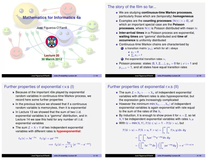
The story of the film so far... We are studying continuous-time - PowerPoint PPT Presentation

The story of the film so far... We are studying continuous-time Markov processes , particularly those which are (temporally) homogeneous Mathematics for Informatics 4a Examples are the counting processes { N ( t ) | t � 0 } , of which an important special case are the Poisson José Figueroa-O’Farrill processes , where N ( t ) is Poisson distributed with mean λt Inter-arrival times in a Poisson process are exponential, waiting times are “gamma” distributed and time of occurrence is uniformly distributed Continuous-time Markov chains are characterised by a transition matrix [ p ij ] , which for all i obeys 1 p ii = 0 � j p ij = 1 Lecture 20 the exponential transition rates ν i 30 March 2012 2 Poisson process: states { 0, 1, 2, ... } , p ij = 0 for j � = i + 1 and p i , i + 1 = 1, and all states have equal transition rates José Figueroa-O’Farrill mi4a (Probability) Lecture 20 1 / 19 José Figueroa-O’Farrill mi4a (Probability) Lecture 20 2 / 19 Further properties of exponential r.v.s (I) Further properties of exponential r.v.s (II) Because of the important rôle played by exponential The sum Z = X 1 + · · · + X n of independent exponential random variables in continuous-time Markov process, we variables with different rates is also hypoexponential, but record here some further properties the expression gets increasingly complicated However the minimum min ( X 1 , . . . , X n ) of independent In the previous lecture we showed that if a continuous random variable is memoryless, then it is exponential exponential variables is again exponential with rate equal to the sum of the rates of the X i In Lecture 13 we showed that the sum of two i.i.d. By induction, it is enough to show prove it for n = 2, so let exponential variables is a “gamma” distribution, and in X , Y be independent exponential variables with rates λ , µ Lecture 14 we saw this held for any number of i.i.d. exponential variables With U = min ( X , Y ) , P ( U � u ) = 1 − P ( U > u ) , but � ∞ � ∞ The sum Z = X + Y of two independent exponential P ( U > u ) = P ( X > u , Y > u ) = f ( x , y ) dx dy variables with different rates is hypoexponential : u u � ∞ � ∞ λµe − λx e − µy dx dy f X ( x ) = λe − λx f Y ( y ) = µe − µy = u u � � ∞ � � � ∞ λµ e − λz − e − µz � � � ⇒ f Z ( z ) = λe − λx dx µe − µy dy = e −( λ + µ ) u = = µ − λ u u José Figueroa-O’Farrill mi4a (Probability) Lecture 20 3 / 19 José Figueroa-O’Farrill mi4a (Probability) Lecture 20 4 / 19

Further properties of exponential r.v.s (III) Birth and death processes (I) The final calculation we will need is P ( X < Y ) for X , Y The only allowed transitions in a counting process are exponential with rates λ , µ those which increase the “population”: n → n + 1 We calculate it by conditioning on X : They are thus said to be “pure birth” processes � ∞ In a “birth and death” process { N ( t ) | t � 0 } we allow P ( X < Y ) = P ( X < Y | X = x ) f X ( x ) dx transitions n → n + 1 (called births ) and n → n − 1 (called 0 � ∞ deaths ), but of course n � 0 P ( X < Y | X = x ) λe − λx dx = Births and deaths are independent and exponentially 0 � ∞ distributed with rates λ n and µ n , respectively, when the P ( x < Y ) λe − λx dx = population is n 0 � ∞ The parameters { λ n | n ∈ N } and { µ n | n ∈ N } are called the e − µx λe − λx dx = birth rates and death rates , respectively 0 � ∞ e −( λ + µ ) x dx A birth and death process is a continuous-time Markov = λ 0 process with states N = { 0, 1, 2, . . . } for which the allowed λ transitions are n → n + 1 and n → n − 1 = λ + µ José Figueroa-O’Farrill mi4a (Probability) Lecture 20 5 / 19 José Figueroa-O’Farrill mi4a (Probability) Lecture 20 6 / 19 Birth and death processes (II) Birth and death processes (III) The transition probabilities are given by p 01 = 1 and µ 1 µ 2 λ 1 + µ 1 λ 2 + µ 2 λ n µ n ( n � 1 ) p n , n + 1 = p n , n − 1 = λ n + µ n λ n + µ n 0 1 2 λ 2 1 λ 1 We argue as follows: p n , n + 1 is the probability that in a λ 1 + µ 1 λ 2 + µ 2 population of n a birth occurs before a death, i.e., P ( B n < D n ) , where B n and D n are the exponential Examples (Pure birth processes) variables corresponding to a birth and death, respectively, pure birth : µ n = 0 for all n � 0 when the population is n . Poisson: µ n = 0 and λ n = λ for all n � 0 Since B n has rate λ n and D n has rate µ n , the results follows from the earlier discussion Yule : µ n = 0 and λ n = nλ for all n � 0, corresponding to a The transition rates are Markov process { N ( t ) | t � 0 } where N ( t ) is the size at time t of a population whose members cannot die, and they give and ( n � 1 ) ν 0 = λ 0 ν n = λ n + µ n birth to new members independently in an exponentially since the time to any transition at population n is distributed amount of time with rate λ min ( B n , D n ) , which is exponential with rate λ n + µ n José Figueroa-O’Farrill mi4a (Probability) Lecture 20 7 / 19 José Figueroa-O’Farrill mi4a (Probability) Lecture 20 8 / 19

Steady-state distribution Example (Linear growth with immigration) Recall that regular discrete-time Markov chains have a This is a model in which µ n = nµ and λ n = nλ + θ , for n � 0 unique steady-state distribution π = ( π n ) , obeying π = πP , Each individual is assumed to give birth at an exponential where P is the transition matrix which evolves the system rate λ one time step. In addition there is an exponential rate of increase θ of the In other words, π is invariant under (discrete) time population due to immigration, so if there are n individuals translations. in the system the total birth rate is nλ + θ Some continuous-time Markov chains also have a unique Deaths occur at an exponential rate µ for each member of steady-state distribution which is invariant under time the population, hence the total death rate for a population translation. of size n is nµ . In other words, π = ( π n ) , where π n ( t + s ) = π n ( t ) , so that is constant in time. A typical question in a birth and death process might be to determine the expectation value E ( N ( t )) of the size of the We will not be concerned with the conditions which population at time t . guarantee the existence and uniqueness of the Usually one derives a differential equation that E ( N ( t )) obeys steady-state distribution. and solves it to determine E ( N ( t )) . We will assume it exists and is unique and we will show how to find it. José Figueroa-O’Farrill mi4a (Probability) Lecture 20 9 / 19 José Figueroa-O’Farrill mi4a (Probability) Lecture 20 10 / 19 For δt small, this is given by Let { N ( t ) | t � 0 } be a continuous-time Markov chain � δt Let n > 0 and consider a small time increment δt : µ n + 1 e − tµ n + 1 dt = 1 − e − µ n + 1 δt ≃ µ n + 1 δt We compute π n ( t + δt ) = P ( N ( t + δt ) = n ) by conditioning 0 on N ( t ) : Similarly, π n ( t + δt ) = P ( N ( t + δt ) = n | N ( t ) = n ) P ( N ( t ) = n ) P ( N ( t + δt ) = n | N ( t ) = n − 1 ) ≃ λ n − 1 δt + P ( N ( t + δt ) = n | N ( t ) = n + 1 ) P ( N ( t ) = n + 1 ) P ( N ( t + δt ) = n | N ( t ) = n ) ≃ 1 − ( λ n + µ n ) δt + P ( N ( t + δt ) = n | N ( t ) = n − 1 ) P ( N ( t ) = n − 1 ) Therefore, Let us focus on one of the conditional probabilities, say, π n ( t + δt ) = ( 1 − δt ( λ n + µ n )) π n ( t ) + µ n + 1 δtπ n + 1 ( t ) P ( N ( t + δt ) = n | N ( t ) = n + 1 ) + λ n − 1 δtπ n − 1 ( t ) This is the probability that a death occurred in ( t , t + δt ] when the population at time t is n + 1 or, said differently, At that population, deaths are exponentially distributed with π n ( t + δt ) − π n ( t ) rate µ n + 1 , so we want the probability of a death in a time ≃ µ n + 1 π n + 1 ( t )+ λ n − 1 π n − 1 ( t )−( λ n + µ n ) π n ( t ) δt interval of length δt at that rate José Figueroa-O’Farrill mi4a (Probability) Lecture 20 11 / 19 José Figueroa-O’Farrill mi4a (Probability) Lecture 20 12 / 19