Scientific Computing I Part I Module 2: Population Modelling - PDF document

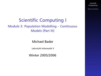
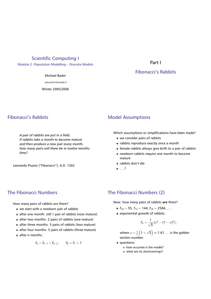
Scientific Computing I Part I Module 2: Population Modelling – Discrete Models Fibonacci’s Rabbits Michael Bader Lehrstuhl Informatik V Winter 2005/2006 Fibonacci’s Rabbits Model Assumptions Which assumptions or simplifications have been made? A pair of rabbits are put in a field. we consider pairs of rabbits If rabbits take a month to become mature rabbits reproduce exactly once a month and then produce a new pair every month, how many pairs will there be in twelve months female rabbits always give birth to a pair of rabbits time? newborn rabbits require one month to become mature rabbits don’t die Leonardo Pisano (“Fibonacci”), A.D. 1202 . . . ? The Fibonacci Numbers The Fibonacci Numbers (2) Now: how many pairs of rabbits are there? How many pairs of rabbits are there? f 10 = 55, f 12 = 144, f 18 = 2584, . . . we start with a newborn pair of rabbits exponential growth of rabbits: after one month: still 1 pair of rabbits (now mature) after two months: 2 pairs of rabbits (one mature) f n = 1 ( φ n − ( 1 − φ ) n ) , √ after three months: 3 pairs of rabbits (two mature) 5 after four months: 5 pairs of rabbits (three mature) √ � � where φ = 1 1 + 5 ≈ 1 . 61 . . . is the golden 2 after n months: section number. questions: f n = f n − 1 + f n − 2 , f 0 = f 1 = 1 how accurate is the model? what are its shortcomings?

Wanted: An improved model Comparison of models Group Work: Discussion: Develop an improved model for the growth of a rabbit population! What are the differences between the proposed models? Model assumptions: 1 Consider: what assumptions do you want to keep the modelling of the rabbits what assumptions do you want to drop or modify the interaction between rabbits Describe your model 2 the environment (time and space) Describe how to run the simulation 3 possible external influences starting conditions evolution of the population . . . Discrete vs. Continuous Models Discrete Population Modeling: count individual rabbits (pairs of rabbits) Part II “clocked” evolution of the population: changes occur at discrete points in time or within Classification of Models time intervalls Continuous Population Modeling: population size ∈ R continuous growth or decay ⇒ population size is a function: p : R → R , p ( x ) = . . . Deterministic vs. Stochastic Models Spatial and Temporal Resolution Spatial resolution, only: Deterministic Population Modeling: population does not grow or decay fixed birth rate, fixed gender distribution expanding and spreading of interest model leads to uniform simulation results Temporal resolution, only: Stochastic Population Modeling: growth and/or decay are of interest probability distribution for birth rate and gender uniform population distribution in a fixed region simulations may lead to different results; both, expected value and aberrations, may be of Temporal and spatial resolution interest how does growth/decay affect population distribution?

Single- vs. Multi-Population Models Level of Detail Rabbit modelling: Single population model: “pair of rabbits” (mature/non-mature) vs. population of rabbits male/female, x years old, healthy/ill, no other species, but distinction between hungry/well-fed, . . . male/female, healthy/ill, hungry/well-fed, . . . ? Spatial resolution: Multi-population: habitat: friendly/hostile environment Example: rabbit population location of food, competitors, predators, . . . competitors: everything that eats carrots!? predators: fox, man, . . . What Quantities have an Effect? prey: carrots what other species have to be included? ⇒ Systems of interacting populations how detailed do we need to model the environment? Finally: What’s the Task? find a solution (find all solutions) find the best solution (optimization problem) analyse solutions: Is it unique? How does it depend on input data? validate the model: quantitatively vs. qualitatively correct?