The Rising Gray Divorce in Japan: Who will Experience the Middle- - PDF document

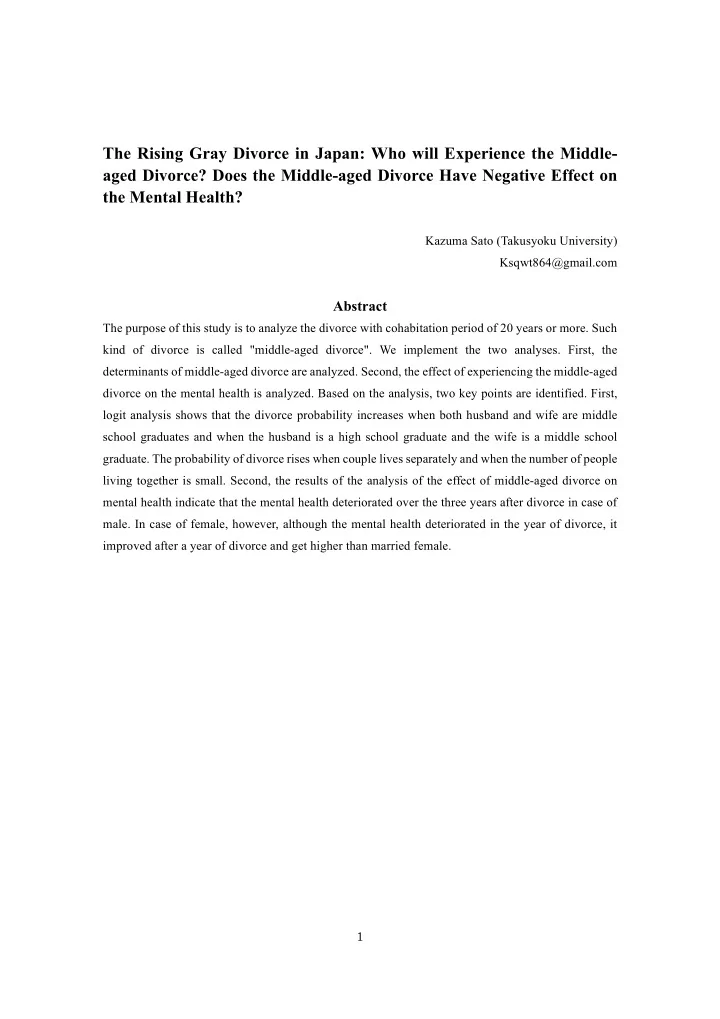
The Rising Gray Divorce in Japan: Who will Experience the Middle- aged Divorce? Does the Middle-aged Divorce Have Negative Effect on the Mental Health? Kazuma Sato (Takusyoku University) Ksqwt864@gmail.com Abstract The purpose of this study is to analyze the divorce with cohabitation period of 20 years or more. Such kind of divorce is called "middle-aged divorce". We implement the two analyses. First, the determinants of middle-aged divorce are analyzed. Second, the effect of experiencing the middle-aged divorce on the mental health is analyzed. Based on the analysis, two key points are identified. First, logit analysis shows that the divorce probability increases when both husband and wife are middle school graduates and when the husband is a high school graduate and the wife is a middle school graduate. The probability of divorce rises when couple lives separately and when the number of people living together is small. Second, the results of the analysis of the effect of middle-aged divorce on mental health indicate that the mental health deteriorated over the three years after divorce in case of male. In case of female, however, although the mental health deteriorated in the year of divorce, it improved after a year of divorce and get higher than married female. 1

1 Motivation Japan has experienced the changes of population dynamics after the collapse of bubble economy. A representative example is the declining birthrate which economists have studied enthusiastically. The other change in population which attracts attention these days is divorce. The number of divorce in Japan has increased after the collapse of bubble economy, and it reached to 289,836 in 2002. However, the number of divorce began to decrease continuously, and it reached to 222,107 in 2014. Although the number of divorce has decreased, percentage of divorce with cohabitation period of 20 years or more has been increasing. Such kind of divorce is called "middle-aged divorce (jyukunen- rikon)". Although it accounted for 3% in total divorce in 1950, it increased to 8% in 1990, 14% in 2000, and 17% in 2014 (Table1). As the number grows, middle-aged divorce has been paid attention gradually. Table 1 Divorce ratio by living period in Japan (%) Living period 1950 1960 1970 1980 1990 2000 2010 2014 Less than 1 year 14.10 17.23 16.36 15.19 9.21 8.35 6.91 6.63 1 year 14.68 18.46 13.45 11.66 8.10 9.19 8.58 7.93 2 year 10.89 14.09 9.87 9.61 7.24 7.88 8.32 7.49 3 year 12.17 9.61 7.73 8.13 6.53 6.68 7.48 6.84 4 year 9.32 5.89 6.57 7.17 6.22 6.04 6.66 6.11 5-9 year 23.36 17.97 22.08 24.37 27.68 21.20 22.95 22.56 10-14 year 8.53 8.80 14.04 12.44 17.32 14.05 13.02 14.72 15-19 year 3.83 4.42 5.53 6.13 9.99 12.73 9.59 10.81 More than 20 year 3.13 3.53 4.38 5.30 7.72 13.88 16.49 16.92 Total 100 100 100 100 100 100 100 100 Source: Ministry of Health, Labor and Welfare “Vital Statistics”. However, there are a few studies about middle-aged divorce, and several important questions has not been answered. For example, who will experience middle-aged divorce? Are there any differences among ordinary divorce and middle-aged divorce? What effect will have on mental health in experiencing the middle-aged divorce? Although these questions are academically and politically interesting due to the increase of old age population in Japan, no studies have examined them. The exception is the Brown and Lin (2013) which examined the middle-aged divorce in United States. The purpose of this paper is to fill the blanks of this field. In order to do so, we implement the two analysis. First, the determinants of middle-aged divorce are analyzed by using random effect logit model. Second, the effect of experiencing the middle-aged divorce on the mental health is analyzed by using matching method. The contributions of this paper are as follow. First, this study focuses on the new trend of divorce in industrialized country by using the data of japan that is the fastest-growing country of aging. Second, we used the biggest panel data of the aged in Japan, Longitudinal Survey of Middle-aged and Elderly 2

Persons, in order to analyze middle-aged divorce. Third, we investigated not only the changes of husband's and wife's employment before and after divorce, but also the changes of activities of hobby, sports and social interaction. Lastly, matching method is used to control the initial differences of individual heterogeneity in examining the effect of divorce on mental health. We employed Entropy Balancing which is developed recently by Hainmueller (2011,2012) and Hainmueller and Xu (2013). The advantage of this method is to be able to control the initial differences of individual heterogeneity almost perfectly. We employed the Entropy Balancing with difference in differences (DID) to control the fixed effect as well as Marcus (2013). Additionally, propensity score matching is also used for the robustness check. 2 Data The data used in the analysis is Longitudinal Survey of Middle-aged and Elderly Persons conducted by Ministry of Health, Labor and Welfare in Japan. This survey was first implemented on 2005 with 33,815 male and female respondents aged 50 to 59 years. The survey is conducted annually, and we use the data from 2005 to 2012. The data investigates families, income, employment, well-being, and type of residence. 3 Estimation method 3.1 The determinants of middle-aged divorce The random effect logit model is estimated to examine the determinants of middles-aged divorce. The econometric model is as follows. ∗ = 𝛾 ' 𝜄 "#)' + 𝛾 + 𝑙 "#)' + 𝛾 - 𝑥 "#)' + 𝛾 / 𝑦 "#)' + 𝜈 " + 𝜁 "# 𝐸 "# 𝐸 "# indicates the divorce dummy which becomes 1 if middle-aged couples divorce, and becomes 0 if otherwise. 𝜄 "#)' indicates the matching of the couples which include husband’s and wife’s educational attainments, the differences between husband' age and wife' age, and the dummy variable which becomes 1 if couples are living separately, and becomes 0 if otherwise. 𝑙 "#)' indicates marriage specific capitals which include children under 20 years old, the number of children, the amount of saving, loan, and home ownership. 𝑥 "#)' indicates the dummy variables of employment of husband and wife which becomes 1 if husband (wife) works and becomes 0 if otherwise. 𝑦 "#)' indicates control variables which include the number of people who live with and year dummy. 3.2 The effect of middle-aged divorce on mental health We briefly explain the method to estimate the average treatment effect on the treated (ATT) using entropy balancing. When estimating the effects of divorce on mental health, the ATT is as follows. 3

A TT = E 𝑍 '" − 𝑍 8" |𝐸 " = 1 = E 𝑍 '" |𝐸 " = 1 − E 𝑍 8" |𝐸 " = 1 (1) In equation (1), 𝑍 " indicates mental health, where 𝑍 ' indicates the value at the time of divorce and 𝑍 8 is the value when the marriage continues. D indicates marriage status. D = 1 indicates that the subjects have recently divorced (treatment group) and D = 0 indicates that the subjects remain married (control group). In (1), E 𝑍 8" |𝐸 " = 1 is the value of mental health that people who remain married would have had had they got divorced, and its value is counterfactual. Entropy balancing solves this problem by using a weighted control group, which can replace E 𝑍 8" |𝐸 " = 1 . 𝑍 8" 𝑥 " "|?@8 E 𝑍 8> |𝐸 > = 1 = (2) 𝑥 " "|?@8 In (2), 𝑥 " is the sampling weight for the control group. It is induced by the constraint equations which satisfy an exact balance between the first and second moments of individual attributes in treatment and control groups. By using the first and second individual attribute moments, both the mean and variance of individual attributes among the treatment and control groups are equated. Entropy balancing can skip the balance check required by PSM and PSW. This is one of the advantages of entropy balancing (Hainmueller and Xu 2013). The analysis exploits the first and second individual attribute moments to equate the mean and variance among the treatment and control groups. The estimation is implemented through two steps. First, sampling weights for the married sample are determined by entropy balancing. Second, OLS is conducted with the sampling weights obtained in the first steps. In the second step, differences in mental health indicators are used as dependent variables to eliminate unobservable fixed effects. We also estimate propensity score matching applying kernel matching for robustness check. The dependent variables are mental health which uses K6. In entropy balancing, we use differences in mental health in the year of divorce (t), one year after getting divorced (t+1), two years after getting divorced (t+2), and three years after getting divorced (t+3), relative to the value of the year prior to divorce (t-1). Same independent variables which are used at logit model are exploited as individual attributes. 4 Result On the basis of the analysis, two key points are identified. First, logit analysis shows that the divorce probability increases when both husband and wife are middle school graduates and when the husband is a high school graduate and the wife is a middle school graduate. Furthermore, the probability of 4