The Power Variance Function Copula Model in Bivariate Survival - PowerPoint PPT Presentation
The Power Variance Function Copula Model in Bivariate Survival Analysis: An application to Twin Data Jose (Pepe) Romeo University of Santiago, Chile jose.romeo@usach.cl Joint work with: Renate Meyer - University of Auckland, New Zealand Diego
The Power Variance Function Copula Model in Bivariate Survival Analysis: An application to Twin Data Jose (Pepe) Romeo University of Santiago, Chile jose.romeo@usach.cl Joint work with: Renate Meyer - University of Auckland, New Zealand Diego Gallardo - University of Sao Paulo, Brazil Workshop on Flexible Models for Longitudinal and Survival Data with Applications in Biostatistics Coventry – UK, July 2015 Pepe Romeo (USAoCH) PVF copula survival analysis Coventry, July 2015 1 / 22
Outline Introduction, some examples of multivariate lifetimes Modeling strategies Copulas The PVF copula model ◮ Definition, particular and limiting cases and dependence properties ◮ Simulating ◮ Estimation Simulation study Application Final comments and future work Pepe Romeo (USAoCH) PVF copula survival analysis Coventry, July 2015 2 / 22
Introduction Survival analysis deals with time-to-event data, e.g. time to death or onset of disease. In multivariate survival analysis there may be a natural association because individuals share biological and/or environmental conditions. Examples: Pepe Romeo (USAoCH) PVF copula survival analysis Coventry, July 2015 3 / 22
Introduction Survival analysis deals with time-to-event data, e.g. time to death or onset of disease. In multivariate survival analysis there may be a natural association because individuals share biological and/or environmental conditions. Examples: ◮ Groups of individuals under to similar environmental conditions ◮ Time to relapse of a disease and time of death, for a subject ◮ Lifetimes of pairs of human organs (e.g. kidneys, eyes) ◮ Recurrent events: asthma attacks for a subject Pepe Romeo (USAoCH) PVF copula survival analysis Coventry, July 2015 3 / 22
Introduction Survival analysis deals with time-to-event data, e.g. time to death or onset of disease. In multivariate survival analysis there may be a natural association because individuals share biological and/or environmental conditions. Examples: ◮ Groups of individuals under to similar environmental conditions ◮ Time to relapse of a disease and time of death, for a subject ◮ Lifetimes of pairs of human organs (e.g. kidneys, eyes) ◮ Recurrent events: asthma attacks for a subject ◮ Clustered failure times such as failure times of twins: to investigate whether the strength of dependence within twin pairs as to the risk of the onset of various diseases is different for MZ and DZ twins (time to appendectomy) Pepe Romeo (USAoCH) PVF copula survival analysis Coventry, July 2015 3 / 22
Introduction Survival analysis deals with time-to-event data, e.g. time to death or onset of disease. In multivariate survival analysis there may be a natural association because individuals share biological and/or environmental conditions. Examples: ◮ Groups of individuals under to similar environmental conditions ◮ Time to relapse of a disease and time of death, for a subject ◮ Lifetimes of pairs of human organs (e.g. kidneys, eyes) ◮ Recurrent events: asthma attacks for a subject ◮ Clustered failure times such as failure times of twins: to investigate whether the strength of dependence within twin pairs as to the risk of the onset of various diseases is different for MZ and DZ twins (time to appendectomy) ➪ The assumption of independence among lifetimes can be unrealistic. ➪ It is of interest to estimate and quantify the dependence among the lifetimes and the effects of covariates under the dependence structure. Pepe Romeo (USAoCH) PVF copula survival analysis Coventry, July 2015 3 / 22
Modeling strategies Shared Frailty Models (random effect models) Clayton (1978), Hougaard (2000), Therneau & Grambsch (2000) Let T ij denote the failure time i -th subject in the j -th cluster, the conditional hazard function is given by iid h ( t | w j , x i ) = h 0 ( t ) exp( β ′ x i ) w j , where e.g., W j ∼ Gamma, Log Normal, . . . Conditional on the frailty term w , the lifetimes are assumed independent, S ( t 1 , . . . , t p | w ) = S ( t 1 | w ) · · · S ( t p | w ) Pepe Romeo (USAoCH) PVF copula survival analysis Coventry, July 2015 4 / 22
Modeling strategies Shared Frailty Models (random effect models) Clayton (1978), Hougaard (2000), Therneau & Grambsch (2000) Let T ij denote the failure time i -th subject in the j -th cluster, the conditional hazard function is given by iid h ( t | w j , x i ) = h 0 ( t ) exp( β ′ x i ) w j , where e.g., W j ∼ Gamma, Log Normal, . . . Conditional on the frailty term w , the lifetimes are assumed independent, S ( t 1 , . . . , t p | w ) = S ( t 1 | w ) · · · S ( t p | w ) Copulas Models (marginal models) Shih & Louis (1995), Duchateau & Janssen (2008), Wienke (2010) F ( t 1 , . . . , t p ) = C α ( F 1 ( t 1 ) , . . . , F p ( t p )) Pepe Romeo (USAoCH) PVF copula survival analysis Coventry, July 2015 4 / 22
Copulas Schweizer & Sklar (1983), Joe (1997), Owzar & Sen (2003), Nelsen (2006) Let T 1 , . . . , T p r.v.’s with T j ∼ F j , j = 1 , . . . , p , and joint cdf F ( t 1 , . . . , t p ) = Pr { T 1 ≤ t 1 , . . . , T p ≤ t p } Pepe Romeo (USAoCH) PVF copula survival analysis Coventry, July 2015 5 / 22
Copulas Schweizer & Sklar (1983), Joe (1997), Owzar & Sen (2003), Nelsen (2006) Let T 1 , . . . , T p r.v.’s with T j ∼ F j , j = 1 , . . . , p , and joint cdf F ( t 1 , . . . , t p ) = Pr { T 1 ≤ t 1 , . . . , T p ≤ t p } Therefore, considering U j = F j ( T j ) ∼ Uniform(0 , 1), F ( t 1 , . . . , t p ) = Pr { U 1 ≤ F 1 ( t 1 ) , . . . , U p ≤ F p ( t p ) } = C α ( F 1 ( t 1 ) , . . . , F p ( t p )) , (1) is called the Copula of the vector ( T 1 , . . . , T p ), it is a multivariate cdf defined on [0 , 1] p with uniformly distributed marginals and α ∈ A is a dependence parameter. Pepe Romeo (USAoCH) PVF copula survival analysis Coventry, July 2015 5 / 22
Copulas Schweizer & Sklar (1983), Joe (1997), Owzar & Sen (2003), Nelsen (2006) Let T 1 , . . . , T p r.v.’s with T j ∼ F j , j = 1 , . . . , p , and joint cdf F ( t 1 , . . . , t p ) = Pr { T 1 ≤ t 1 , . . . , T p ≤ t p } Therefore, considering U j = F j ( T j ) ∼ Uniform(0 , 1), F ( t 1 , . . . , t p ) = Pr { U 1 ≤ F 1 ( t 1 ) , . . . , U p ≤ F p ( t p ) } = C α ( F 1 ( t 1 ) , . . . , F p ( t p )) , (1) is called the Copula of the vector ( T 1 , . . . , T p ), it is a multivariate cdf defined on [0 , 1] p with uniformly distributed marginals and α ∈ A is a dependence parameter. From (1) the joint pdf is given by p � f ( t 1 , . . . , t p ) = c α ( F 1 ( t 1 ) , . . . , F p ( t p )) f j ( t j ) j =1 Pepe Romeo (USAoCH) PVF copula survival analysis Coventry, July 2015 5 / 22
Archimedean Copulas Genest & MacKay (1986), Joe (1997), Nelsen (2006). A copula C α is called Archimedean if there exists a convex function ϕ − 1 : [0 , ∞ ] �→ [0 , 1] , so that the copula C α can be written as α C α ( u 1 , u 2 ) = ϕ − 1 α ( ϕ α ( u 1 ) + ϕ α ( u 2 )) , for all ( u 1 , u 2 ) ∈ [0 , 1] 2 and α ∈ A . Pepe Romeo (USAoCH) PVF copula survival analysis Coventry, July 2015 6 / 22
Archimedean Copulas Genest & MacKay (1986), Joe (1997), Nelsen (2006). A copula C α is called Archimedean if there exists a convex function ϕ − 1 : [0 , ∞ ] �→ [0 , 1] , so that the copula C α can be written as α C α ( u 1 , u 2 ) = ϕ − 1 α ( ϕ α ( u 1 ) + ϕ α ( u 2 )) , for all ( u 1 , u 2 ) ∈ [0 , 1] 2 and α ∈ A . ➪ when ϕ − 1 corresponds to the Laplace transform of W in a multiplicative frailty model h ( t | w ) = h 0 ( t ) w , copula models induced by frailty models are Archimedean copulas (Oakes, 1989), e.g: Pepe Romeo (USAoCH) PVF copula survival analysis Coventry, July 2015 6 / 22
Archimedean Copulas Genest & MacKay (1986), Joe (1997), Nelsen (2006). A copula C α is called Archimedean if there exists a convex function ϕ − 1 : [0 , ∞ ] �→ [0 , 1] , so that the copula C α can be written as α C α ( u 1 , u 2 ) = ϕ − 1 α ( ϕ α ( u 1 ) + ϕ α ( u 2 )) , for all ( u 1 , u 2 ) ∈ [0 , 1] 2 and α ∈ A . ➪ when ϕ − 1 corresponds to the Laplace transform of W in a multiplicative frailty model h ( t | w ) = h 0 ( t ) w , copula models induced by frailty models are Archimedean copulas (Oakes, 1989), e.g: ◮ W ∼ Gamma then ( U 1 , U 2 ) ∼ Clayton copula ◮ W ∼ Positive Stable then ( U 1 , U 2 ) ∼ Gumbel copula ◮ W ∼ Inverse Gaussian then ( U 1 , U 2 ) ∼ Inverse Gaussian copula Pepe Romeo (USAoCH) PVF copula survival analysis Coventry, July 2015 6 / 22
Copulas Kendall’s tau Let ( T 1 , T 2 ) a continuous r.v. with copula C α , then the Kendall’s tau coefficient for ( T 1 , T 2 ) is given by �� τ α = 4 [0 , 1] 2 C α ( u 1 , u 2 ) dC α ( u 1 , u 2 ) − 1 Pepe Romeo (USAoCH) PVF copula survival analysis Coventry, July 2015 7 / 22
Copulas Kendall’s tau Let ( T 1 , T 2 ) a continuous r.v. with copula C α , then the Kendall’s tau coefficient for ( T 1 , T 2 ) is given by �� τ α = 4 [0 , 1] 2 C α ( u 1 , u 2 ) dC α ( u 1 , u 2 ) − 1 For Archimedean copulas, Kendall’s tau is written as � 1 ϕ α ( t ) τ α = 4 α ( t ) dt + 1 ϕ ′ 0 Pepe Romeo (USAoCH) PVF copula survival analysis Coventry, July 2015 7 / 22
The PVF (Power variance function) distribution W ∼ PVF( α, δ, θ ) for α ∈ (0 , 1), δ > 0, and θ ≥ 0 if for w > 0 the pdf is given by Pepe Romeo (USAoCH) PVF copula survival analysis Coventry, July 2015 8 / 22
Recommend
More recommend
Explore More Topics
Stay informed with curated content and fresh updates.
![Variance = E[I 2 ] 2pE[I] + p 2 = E[I] 2p p + p 2 = 2 2 = p-2p+ p pq variance.1](https://c.sambuz.com/1069957/variance-s.webp)
