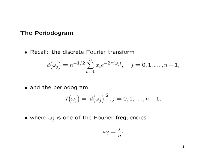
The Periodogram Recall: the discrete Fourier transform n = n 1 / 2 - PowerPoint PPT Presentation

The Periodogram • Recall: the discrete Fourier transform n = n − 1 / 2 x t e − 2 πiω j t , � � � d ω j j = 0 , 1 , . . . , n − 1 , t =1 • and the periodogram 2 , j = 0 , 1 , . . . , n − 1 , � �� � � � I ω j = � d ω j � � � • where ω j is one of the Fourier frequencies ω j = j n. 1

Sine and Cosine Transforms • For j = 0 , 1 , . . . , n − 1, n � � = n − 1 / 2 x t e − 2 πiω j t � d ω j t =1 n n = n − 1 / 2 − i × n − 1 / 2 � � � � � � x t cos 2 πω j t x t sin 2 πω j t t =1 t =1 � � � � = d c ω j − i × d s ω j . � � � � • d c ω j and d s ω j are the cosine transform and sine trans- form , respectively, of x 1 , x 2 , . . . , x n . � 2 + d s � 2 . � � � � • The periodogram is I ω j = d c ω j ω j 2

Sampling Distributions • For convenience, suppose that n is odd: n = 2 m + 1. • White noise: orthogonality properties of sines and cosines mean that d c ( ω 1 ), d s ( ω 1 ), d c ( ω 2 ), d s ( ω 2 ), . . . , d c ( ω m ), d s ( ω m ) have zero mean, variance 1 2 σ 2 w , and are uncorrelated. • Gaussian white noise: d c ( ω 1 ), d s ( ω 1 ), d c ( ω 2 ), d s ( ω 2 ), . . . , � 0 , 1 � 2 σ 2 d c ( ω m ), d s ( ω m ) are i.i.d. N . w � � ∼ 1 2 σ 2 w × χ 2 • So for Gaussian white noise, I ω j 2 . 3

• General case: d c ( ω 1 ), d s ( ω 1 ), d c ( ω 2 ), d s ( ω 2 ), . . . , d c ( ω m ), d s ( ω m ) have zero mean and are approximately uncorrelated, and ≈ 1 � � �� � � �� � � var d c ω j ≈ var d s ω j 2 f x ω j , � � where f x ω j is the spectral density function. • If x t is Gaussian, � 2 + d s � 2 � � � � I x ω j d c ω j ω j ∼ approximately χ 2 � = 2 , 1 � 1 � � 2 f x ω j 2 f x ω j and I x ( ω 1 ), I x ( ω 2 ), . . . , I x ( ω m ) are approximately indepen- dent. 4

Spectral ANOVA • For odd n = 2 m + 1, the inverse transform can be written m 2 � � � � � � � � �� � x t − ¯ x = d c ω j cos 2 πω j t + d s ω j sin 2 πω j t . √ n j =1 • Square and sum over t ; orthogonality of sines and cosines implies that n m � 2 + d s � 2 � � x ) 2 = 2 � � � � ( x t − ¯ d c ω j ω j t =1 j =1 m � � � = 2 I ω j . j =1 5

ANOVA table: Source df SS MS 2 2 I ( ω 1 ) ω 1 I ( ω 1 ) 2 2 I ( ω 2 ) ω 2 I ( ω 2 ) . . . . . . . . . . . . ω m 2 2 I ( ω m ) I ( ω m ) x ) 2 Total 2 m = n − 1 � ( x t − ¯ 6

Hypothesis Testing • Consider the model � � x t = A cos 2 πω j t + φ + w t . • Hypotheses: – H 0 : A = 0 ⇒ x t = w t , white noise; – H 1 : A > 0, white noise plus a sine wave. • Note: no autocorrelation in either case. 7

• Two cases: – ω j known: use � � I ω j F j = � � ( m − 1) − 1 � j ′ � = j I ω j ′ which is F 2 , 2( m − 1) under H 0 . – ω j unknown: use max( F 1 , F 2 , . . . , F m ), or equivalently � � � � max I ω j , j = 1 , 2 , . . . , n κ = � � m − 1 � j I ω j and � � �� − ξ ( m − 1 − log m ) P( κ > ξ ) ≈ 1 − exp − m exp . m − ξ 8

Example: the Southern Oscillation Index • Using SAS: proc spectra program and output. • Using R: par(mfcol = c(2, 1)) # Use fft() to calculate the periodogram directly; note that # frequencies are expressed in cycles per year, and the # periodogram values are similarly scaled by 12: freq = 12 * (0:(length(soi) - 1)) / length(soi) plotit = (freq > 0) & (freq <= 6) soifft = fft(soi) / sqrt(length(soi)) plot(freq[plotit], Mod(soifft[plotit])^2 / 12, type = "l") # Use spectrum(); override some defaults to make it match: spectrum(soi, log = "no", fast = FALSE, taper = 0, detrend = FALSE) 9