The JPEG Standard, "Main Profile" For simplicity, assume - - PowerPoint PPT Presentation

• 1 -

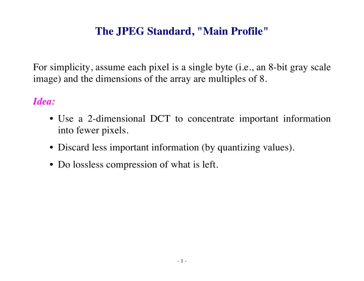
The JPEG Standard, "Main Profile"

For simplicity, assume each pixel is a single byte (i.e., an 8-bit gray scale image) and the dimensions of the array are multiples of 8. Idea:

• Use a 2-dimensional DCT to concentrate important information

into fewer pixels.

• Discard less important information (by quantizing values).
• Do lossless compression of what is left.

• 2 -

Step 1

• Subtract 128 from each pixel.
• Now the pixel values go from –127 to +127 rather than from 0 to

255.

• Although not necessary from a mathematical point of view, this is

a "natural" level shift from a signal processing point of view, and in practice reduces the precision requirements for the DCT computation.

• 3 -

Step 2

• Partition the image into 8 by 8 sub-images.
• Perform independent two dimensional DCT's on each of these

sub-images.

• Each resulting 8 x 8 matrix will have values in the range -1,023

to + 1,023.

• 4 -

Step 3

• Quantize all coefficients of a transformed sub-image according

to an 8 by 8 table of quantization step sizes.

• That is, if the (i,j)th entry of the table is q, then a value x in the

(i,j)th position of a transformed sub-image is adjusted by doing: x := round_to_nearest_integer(x/q) Example: The lumininence quantization matrix suggested in the JPEG standard (Table K.1); these entries can be divided by 2 for better quality.

16 11 10 16 24 40 51 61 12 12 14 19 26 58 60 55 14 13 16 24 40 57 69 56 14 17 22 29 51 87 80 62 18 22 37 56 68 109 103 77 24 35 55 64 81 104 113 92 49 64 78 87 103 121 120 101 72 92 95 98 112 100 103 99

• 5 -

Step 4

• The DC coefficients are the values in position (0,0) of each

transformed sub-image; they are the average intensity of the sub- image.

• They are encoded by representing each as the difference between

it and the one in the preceding block.

• These differences are then represented as (size, amplitude) pairs,

where 0 ≤ size ≤ 11 specifies the number of bits that are used to represent the amplitude, which uses a one's complement representation (i.e., positive values use a normal binary representation and negative values use the normal representation with each bit complemented).

• The sizes are then Huffman coded with the amplitudes appended

(the Huffman code table can be specified).

• 6 -

(DC Sizes from the JPEG Standard)

• 7 -

Step 5

• The AC coefficients of each 8 x 8 transformed sub-image are all

values except for the one in position (0,0).

• Traverse them in a zig-zag order going from the upper left down

to the lower right corner.

• Each non-zero coefficient of the zig-zag traversal is encoded as a

(run, size, amplitude) triple, where 0 ≤ run ≤ 15 is the number of zero coefficients preceding it; use (15,0,–) as many times as necessary to represent runs of 16 or more 0's.

• Reserve (0,0,–) to indicate that all remaining AC coefficients in

the transformed sub-block are 0.

• The (run, size) values are Huffman coded with the amplitudes

appended (using size bits in one's complement representation).

• The Huffman code table can be specified, and can be different

from the one used for the DC coefficients.

• 8 -

(AC Sizes from the JPEG Standard)

• 9 -

Details of Zig-Zag Order

Let X be a n by n matrix where X[0,0] is the upper left corner and X[n–1,n–1] is the lower right corner. The Zig-Zag traversal visits X from the upper left down to the lower right. There are two symmetric versions; JPEG uses the "odd" version:

• 10 -

Example: Suppose X contained the numbers 1 through 64 in row major order:

1 2 3 4 5 6 7 8 9 10 11 12 13 14 15 16 17 18 19 20 21 22 23 24 25 26 27 28 29 30 31 32 33 34 35 36 37 38 39 40 41 42 43 44 45 46 47 48 49 50 51 52 53 54 55 56 57 58 59 60 61 62 63 64

Then the (odd) ZigZag traversal is:

1, 2, 9, 17, 10, 3, 4, 11, 18, 25, 33, 26, 19, 12, 5, 6, 13, 20, 27, 34, 41, 49, 42, 35, 28, 21, 14, 7, 8, 15, 22, 29, 36, 43, 50, 57, 58, 51, 44, 37, 30, 23, 16, 24, 31, 38, 45, 52, 59, 60, 53, 46, 39, 32, 40, 47, 54, 61, 62, 55, 48, 56, 63, 64

• 11 -

ZigZag Algorithm Let Z[0] ... Z[2n–1] be the array to place the elements of X in zig-zag order:

• On any given diagonal, the sum of the two indices is the same; the index i is this sum,

going from 0 to 2(n–1).

• The index j goes from 0 to i on the diagonals 0 through n–1, then on diagonal n it

starts at 1, on diagonal n+1 it starts at 2, ..., and on diagonal 2(n–1), which contains

• nly the entry (n–1,n–1), it starts at n-1.
• So the the starting and ending values for j have to be reduced by 1 each time as i goes

from n to 2(n–1). Below is the traversal algorithm for an odd ZigZag; for the symmetric "even" version that starts 1, 9, 2, 3, 10, 17, ..., just change the "odd" to "even" in the if statement: index = –1 for i=0 to 2(n–1) do if (i < n) then bound=0 else bound = i–n+1 for j=bound to i–bound do begin index = index+1 if i is odd then Z[index] = X[j,i–j] else Z[index] = X[i–j,j] end end

• 12 -

Pre-Computation Of The Zig-Zag Order

Idea: Since the order doesn't change and we are only computing it for 64 values, compute it once and store it in an 8x8 matrix. Compute a translation matrix M that can be used each time an 8x8 array X has to be traversed in zig-zag order. For example, modify the algorithm

• f the previous page to change the inner if statement to:

if i is odd then M[j, i–j] = index else M[i–j, j] = index Now, each time we need to compute the zig-zag array Z for an 8x8 matrix X, we can simply do these 64 assignment statements: Z[M[i,j]] = X[i,j], 0 ≤ i,j ≤ 7