Image and Video Coding: From Block Transforms to JPEG JPEG Overview - PowerPoint PPT Presentation
Image and Video Coding: From Block Transforms to JPEG JPEG Overview The JPEG Standard Joint Photographic Experts Group (JPEG) Standard is named after the group which created it Joint committee of ITU-T and ISO/IEC JTC 1 ITU-T Study Group 16,
Image and Video Coding: From Block Transforms to JPEG
JPEG Overview The JPEG Standard Joint Photographic Experts Group (JPEG) Standard is named after the group which created it Joint committee of ITU-T and ISO/IEC JTC 1 ITU-T Study Group 16, Working Party 3, Question 6 (Visual Coding Experts Group: VCEG) ISO/IEC Joint Technical Committee 1, Subcommittee 29, Working Group 1 (JTC 1/SC 29/WG 1) Digital Compression and Coding of Continuous-Tone Still Images (JPEG Standard) Officially ITU-T Recommendation T.81 and International Standard ISO/IEC 10918-1 Commonly referred to as JPEG Specifies compression for gray-level and color images Work commences in 1986 Standard published in 1992 Still most widely used standard for image compression Heiko Schwarz (Freie Universität Berlin) — Image and Video Coding: From Block Transforms to JPEG 2 / 43
JPEG Overview / Color Components JPEG: Source Image Formats Single-Component Images 2D array of integer sample values Characterized by single component image width W and image height H range [ 0 ; 2 B − 1 ] sample bit depth B Multi-Component Images / Color Images most common: Y’CbCr 4:2:0 Multiple 2D arrays of integer sample values Characterized by Cb Maximum width W and height H of arrays Vertical and horizontal downsampling factors Y’ Most common: Y’CbCr format Cr Y’: Full-resolution luma components Cb, Cr: Downsampled chroma components Heiko Schwarz (Freie Universität Berlin) — Image and Video Coding: From Block Transforms to JPEG 3 / 43
JPEG Overview / Partitioning JPEG: Color Components and Partitioning Partitioning of Color Components Each color components is partitioned into 8 × 8 blocks of samples If arrays size is not a multiple of 8 × 8: Insert missing samples (will be removed after decoding) Most common method: Constant border extension s [ x , y ] = s [ W − 1 , y ] s [ x , y ] = s [ x , H − 1 ] Heiko Schwarz (Freie Universität Berlin) — Image and Video Coding: From Block Transforms to JPEG 4 / 43
JPEG Overview / Source Coding Algorithm JPEG: Basic Source Coding Algorithm sample array lossy part original entropy bits 2d block quantization quantization bitstream coding transform 8 × 8 block transmission or storage sample array reconstructed entropy bits 2d inverse dequantization bitstream decoding transform 8 × 8 block Basic Encoding Algorithm (for 8 × 8 blocks of samples) 1 Transform : Energy compaction (reduce statistical dependencies between samples) 2 Quantization : Approximate signal in a suitable way (enables more efficient coding) 3 Entropy Coding : Represent quantization indexes with as less bits as possible Decoder : Inverse operations of encoder (note: quantization is not invertible) Heiko Schwarz (Freie Universität Berlin) — Image and Video Coding: From Block Transforms to JPEG 5 / 43
Block Transform / Linear Transform Linear Transform of Sample Vectors Consider arbitrary vector s = ( s 0 , s 1 , s 2 , · · · , s N − 1 ) T of N samples Linear transform : Matrix-vector multiplication (each coefficient = linear combination of samples) Forward Transform (in encoder) u A s Map sample vector s to vector u of transform coefficients = · A : N × N transform matrix u = A · s with u : vector with N coefficients Inverse Transform (in decoder) A − 1 s ′ u ′ Map reconstructed coefficients u ′ to sample vector s ′ A − 1 : inverse of matrix A = · s ′ = A − 1 · u ′ with u ′ : N reconstructed coefficients Perfect reconstruction ( s ′ = s ) in the absence of quantization ( u ′ = u ) Heiko Schwarz (Freie Universität Berlin) — Image and Video Coding: From Block Transforms to JPEG 6 / 43
Block Transform / Linear Transform Interpretation of Linear Transforms Inverse Transform Reconstructed vector of samples is obtained by s ′ = A − 1 · u ′ u ′ 0 u ′ 1 = u ′ 0 · b 0 + u ′ 1 · b 1 + u ′ 2 · b 2 + · · · + u ′ = · N − 1 · b N − 1 s ′ b 0 b 1 b 2 · · · b N − 1 . . . u ′ N − 1 Reconstructed vector s ′ is represented as linear combination of basis vectors b k (columns of A − 1 ) Transform coefficients u ′ k represent weighting factors for corresponding basis vectors b k Forward Transform Vector of transform coefficients is obtained by u = A · s Decomposition of sample vector s into linear combination of basis vectors b k Transform coefficients u k represent the corresponding weighting factors Heiko Schwarz (Freie Universität Berlin) — Image and Video Coding: From Block Transforms to JPEG 7 / 43
Block Transform / Linear Transform Example for Possible Basis Vectors Linear independent basis vectors (required for invertibility of A and A − 1 ) 1 3 1 1 1 1 − 1 − 1 b 0 = b 1 = b 2 = b 3 = , , , 1 − 1 − 1 1 1 − 3 1 − 1 Inverse transform matrix A − 1 1 3 1 1 1 1 − 1 − 1 A − 1 = b 0 b 1 b 2 b 3 = 1 − 1 − 1 1 1 − 3 1 − 1 Forward transform matrix A 0 . 250 0 . 250 0 . 250 0 . 250 A − 1 � − 1 = 0 . 125 0 . 125 − 0 . 125 − 0 . 125 � A = 0 . 250 − 0 . 250 − 0 . 250 0 . 250 0 . 125 − 0 . 375 0 . 375 − 0 . 125 Heiko Schwarz (Freie Universität Berlin) — Image and Video Coding: From Block Transforms to JPEG 8 / 43
Block Transform / Orthogonal Transform Orthogonal Transform Mean Squared Error (MSE) of Samples 1 1 1 � 2 = � T � T � s ′ − s s ′ − s A − 1 u ′ − A − 1 u A − 1 u ′ − A − 1 u � s ′ � � � � � � k − s k = N N N k 1 �� T A − 1 � T · u ′ − u A − 1 � u ′ − u � � � � = · N In general: Complicated relationship to quantization errors u ′ k − u k of transform coefficients MSE cannot be minimized by independent quantization of transform coefficients Orthogonal Transforms Inverse matrix is equal to the transpose: A − 1 = A T MSE in sample domain is equal to MSE in transform domain 1 � 2 = 1 � � � 2 � s ′ � u ′ k − s k k − u k N N k k Transform coefficients can be quantized independently of each other Main reason for using orthogonal transforms in lossy coding Heiko Schwarz (Freie Universität Berlin) — Image and Video Coding: From Block Transforms to JPEG 9 / 43
Block Transform / Orthogonal Transform Orthonormal Basis Property of Orthogonal Transforms Consider product of forward and inverse matrix: A · A T = A · A − 1 = I b 0 1 0 0 0 · · · b 1 0 1 0 0 · · · b 2 0 0 1 0 b 0 b 1 b 2 · · · b N − 1 · · · = · . . . . . ... . . . . . . . . . . b N − 1 0 0 0 1 · · · Basis vectors b k are orthogonal to each other Basis vectors b k have a length equal to 1 Basis vectors of orthogonal matrices form an orthonormal basis Geometric Interpretation Rotation (and possible reflection) of coordinate system Heiko Schwarz (Freie Universität Berlin) — Image and Video Coding: From Block Transforms to JPEG 10 / 43
Block Transform / Orthogonal Transform Example of an Orthogonal Transform for N = 2 Vector of two samples s = ( s 0 , s 1 ) T Inverse transform matrix s 1 � 1 � � 1 � 1 A − 1 = b 0 b 1 = √ 1 − 1 u 0 · b 0 2 Representation of signal vector s = u 0 · b 0 + u 1 · b 1 b 0 � 1 s � � � � � 4 = u 0 · 1 + u 1 · 1 1 √ √ 2 1 − 1 2 2 s 0 � 4 � 1 b 1 � � � � 1 u 1 · b 1 = 3 · + 1 · 2 1 − 1 Forward transform: Project signal vector onto basis vectors √ √ u 0 = b T u 1 = b T 0 · s = 3 2 and 1 · s = 2 Heiko Schwarz (Freie Universität Berlin) — Image and Video Coding: From Block Transforms to JPEG 11 / 43
Block Transform / Decorrelation Goal of Transform joint histogram of two adjacent samples 15 test images (each 768 × 512) N ( s n , s n + 1 ) s n + 1 s n Goal of Transform: Compaction of Signal Energy Reduce statistical dependencies between samples inside block ! Linear transforms can only remove linear dependencies Heiko Schwarz (Freie Universität Berlin) — Image and Video Coding: From Block Transforms to JPEG 12 / 43
Block Transform / Decorrelation Statistical Measures for Characterizing Linear Dependencies Consider collection of one-dimensional signals (interpreted as realization of random source) Consider two samples with fixed spatial relationship s [ k ] and s [ ℓ ] Associated random variables are denoted as S k and S ℓ Covariance and Correlation Coefficient σ 2 ( S k − µ k ) 2 � � Variance and Mean: k = E µ k = E { S k } σ 2 � � ( σ 2 k , k = σ 2 Covariance: k ,ℓ = E ( S k − µ k ) ( S ℓ − µ ℓ ) k ) σ 2 k ,ℓ Correlation coefficient: ̺ k ,ℓ = ( − 1 ≤ ̺ k ,ℓ ≤ 1 ) � σ 2 k · σ 2 ℓ Interpretation σ 2 No linear dependencies: ̺ k ,ℓ = 0 and k ,ℓ = 0 (decorrelated samples) Strong linear dependencies: | ̺ k ,ℓ | � 1 Heiko Schwarz (Freie Universität Berlin) — Image and Video Coding: From Block Transforms to JPEG 13 / 43
Recommend
More recommend
Explore More Topics
Stay informed with curated content and fresh updates.

![Image and Video Coding: Hybrid Video Coding s n 1 [ x , y ] s n [ x , y ] m k = ( m x , m](https://c.sambuz.com/761427/image-and-video-coding-hybrid-video-coding-s.webp)
