The Impact of Conditional Cash transfers programmes on household - PowerPoint PPT Presentation
The Impact of Conditional Cash transfers programmes on household work decisions in Ghana. By E.E-A. Mochiah , R.D. Osei & I.O. Akoto Outline Introduction Objectives Evidence from other studies LEAP program Methodology
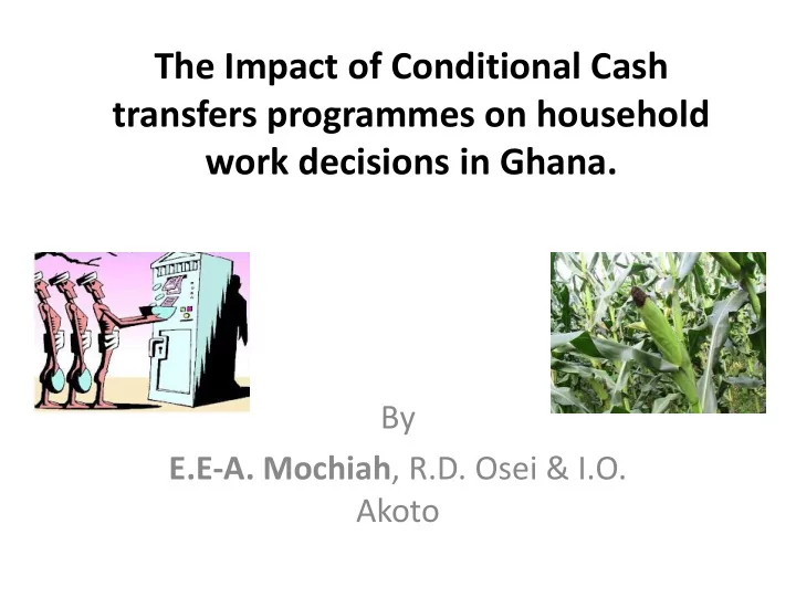
The Impact of Conditional Cash transfers programmes on household work decisions in Ghana. By E.E-A. Mochiah , R.D. Osei & I.O. Akoto
Outline • Introduction – Objectives • Evidence from other studies – LEAP program • Methodology • Results/Findings • Conclusions • Recommendations
Introduction • In the last decade, CCT programs have been very popular in developing countries as a policy tool to increase human capital. • Argument of CCTs creating disincentives to work . • CCT programs provide cash payments to households conditional on regular school attendance and visiting health clinics among others. – CCTs have achieved quantified success in reaching the poor and bringing about short-term improvements in consumption, education, and health (Schultz 2004; Gertler 2004; Rawlings and Rubio 2003),
Evidence in favour of CCTs • Skoufias and Maro (2008), assesses the impact of Mexico’s PROGRESA programme on poverty and adult work incentives. – PROGRESA’s cash transfers have not discouraged people from working • Ardington et al. (2009) concludes that – large cash transfers (pensions in South Africa) to the elderly lead to increased employment among prime-aged adults, which occurs primarily through labor migration. • Ferro et al. (2010) find that the Bolsa Escola CCT program in Brazil – increased mothers’ and fathers’ probability of participation in labour force work. • Oliveira et al., 2007 finds in Brazil’s Bolsa Família that – Women in benefiting households had labour market participation rates 4.3 percentage points higher than women in non-participating households
Evidence Against CCTs • Maluccio and Flores (2005) used Nicaragua’s “Red de Proteccion Social" conditional cash transfer scheme. – find no effect on labour supply • Bertrand et al. (2003) use cross-sectional data in South Africa and estimate that – pension receipt substantially lowers the labor market participation of working-age adults in the household.
What of Ghana’s LEAP? • Specifically, the objectives of this paper is to find out whether or not – Conditional Cash Transfer scheme has increased households total hours worked (labour supply) generally; – The hours worked on farm (agriculture) ,off-farm (non- farm enterprise) and paid employment has increased with the CCT scheme
LEAP in Ghana • Provides cash and health insurance to extremely poor households across Ghana – to alleviate short-term poverty and – encourage long term human capital development. • Aimed at improving the basic consumption of beneficiary households by – increasing school enrolment, attendance and retention of children, – improving on livelihood income-earned activities like farming. GLSS5- 164,370 households (bottom 20% of extremely poor • households in Ghana) The target group includes • subsistence farmers and fisher folk, – extremely poor citizens above 65 years without any subsistence support – persons living with severe disabilities without any productive capacity; – Care Givers of OVCs-orphans and vulnerable children (particularly Children Affected By AIDS • and children with severe disabilities), Incapacitated/extremely poor people living with HIV/AIDS and • Pregnant Women/Lactating Mothers with HIV/AIDS. •
LEAP..cont’d For the aged and persons with severe disabilities, the cash transfer • is unconditional. As at 2008,each beneficiary receives GH¢8.00 and that could • increase to GH¢15,00 , depending on the number of beneficiaries in the family (to a maximum of four)- 2(GH¢10),3(GH¢12),4 or more(GH¢15)- Exchange rate at 2008 was about $1 to GH¢1 In July 2012, this was revised to GH¢12 to GH¢36 during a re- • launch. Exchange rate at 2012 was $1 to GH¢1.88 Some recent contributions have came from DFID (£36.4 million), • World Bank (US$20 million), GoG (GH¢18 million)-July 2012 As at 2010 coverage was 35,000 HH but has increased to 71,456 HH • in 2013 (98 districts) with a target of 150,000 HH in 2014 and 200,000 HH in 2015 (170 districts) Amount was to be adequate and acceptable so not to • – encourage unemployment, – create dependency or – benefit beneficiary households excessively compared to the other income groups in the community
Methodology The sampling strategy of the LEAP programme entailed a • longitudinal propensity score matching (PSM) design. The PSM strategy enables one to attribute changes over time • to the intervention by allowing for the construction of a counterfactual through the matched comparison group Group LEAP(Treatment) YALE(Control) Survey Baseline Follow up Baseline Follow up Period 2010 2012 2010 2012 No of HH 700 646 5009 858
Methodology cont’d • Any significant effect of the cash transfer on household hours worked between the treatment group and the control group? – overall, for agriculture, paid employment and non- farm enterprise. • To do this, we adopt difference-in-difference method – vastly used in literature to account for differences in outcome variables in randomized experiments.
• Y it = β 0 + β 1 T it + β 2 A it + β 3 T it A it +β 4 X it + ε it (1) • Where Y it is the number of hours worked by the household i at time t (t=1, 2), • X it is a vector containing covariates which may influence the number of hours worked by a household. • T it is a trend variable (= 1 in follow up and zero (0) for the baseline period. • A it is the treatment dummy • T it A it is an interactive variable . • The coefficient of this interactive variable provides a measure of effect of the intervention which is referred to as the difference in difference estimator and can be expressed as : • β 3 = (Y* a1 -Y* c1 )-(Y* a2 -Y* c2 ) (2)
Descriptive Results Sex of Household head Dist. of age of HH head Male 45.5 10-19 1.0 Female 54.5 20-29 5.6 Marital status of Household head 30-39 12.0 Married 42.0 40-49 13.0 Consensual Union 5.9 50-59 17.3 Separated 4.0 60-64 6.7 Divorced 11.1 65+ 44.5 Widowed 32.6 Household size Never Married 4.5 1 18.9 Betrothed 0.0 2-3 32.7 Educational level of head 4-5 24.5 No education 46.5 6-7 15.3 Senior High School and below 49.4 8-9 5.9 Above Senior High School 4.1 10+ 2.7 Mean household size 3.9 Average HH size is 3.9 Sex of household heads was 54.5 for women
Annual Average labour hours/Days per household Labour Hours Baseline Follow-up Treatment Control Treatment Control Agric 306.1 671.2 349.6 550.5 Paid employment 95.1 106.6 108.4 78.9 Non-farm Enterprise 640.3 673.9 655.9 836.2 Total 1041.5 1451.7 1113.8 1465.7 Days per HH Agric 38 84 44 69 Paid employment 12 13 14 10 Non-farm Enterprise 80 84 82 105 Total 130 181 139 183
Analytical Results Total labour hrs Agriculture Paid employment Non-farm Enterprise Eqn1 Eqn2 Eqn3 Eqn4 Eqn5 Eqn6 Eqn7 Eqn8 VARIABLES lTotallabhrs lTotagriclabhrs lTpaidemphrswk lTotlabhrs_ent Treatdum -0.823*** -0.070 -0.914*** -0.111 -0.075 -0.202** -0.099 0.042 (0.153) (0.117) (0.149) (0.111) (0.085) (0.086) (0.164) (0.165) Time2 0.659*** 0.540** 0.564*** 0.678*** -0.052 0.200 0.366** -0.006 (0.147) (0.245) (0.143) (0.230) (0.082) (0.177) (0.158) (0.296) Treattime -0.398* 0.263 -0.489** -0.074 0.160 0.315* -0.218 0.110 (0.216) (0.264) (0.211) (0.249) (0.120) (0.191) (0.232) (0.371) -0.121*** lLabannualinc 0.389*** -0.140*** (0.024) (0.026) (0.036) 0.044 HHhasnonfarm 0.287 -0.223* (0.174) (0.184) (0.133) -0.095*** lEnt_sales1 0.348*** -0.003 (0.017) (0.018) (0.013) lagricincome 0.219*** -0.043*** -0.039 (0.018) (0.013) (0.026) 0.018 lLoanamt 0.001 0.032** 0.121*** (0.018) (0.019) (0.014) (0.027) -0.004 lLendamt -0.044 0.077*** 0.265*** (0.027) (0.029) (0.021) (0.041) -0.061*** lTransfers -0.095*** -0.045*** -0.074*** (0.017) (0.018) (0.013) (0.025) -0.098*** TTlTransfer -0.101** -0.101*** -0.006
(0.040) (0.038) (0.029) (0.056) lCompensatn_wage -0.028 0.050 -0.185*** -0.013 (0.046) (0.043) (0.033) (0.065) cancarryload 0.845*** 0.725*** 0.594*** 1.129*** (0.117) (0.110) (0.086) (0.163) lsize 1.274*** 2.851*** -0.139** -0.596*** (0.088) (0.072) (0.065) (0.123) males_in_hh 0.012 0.388*** 0.414*** -0.437*** (0.092) (0.086) (0.066) (0.129) hhsize 0.101*** 0.119*** 0.043*** 0.110*** (0.021) (0.020) (0.015) (0.029) HHelectricity -0.077 -0.139* 0.072 0.688*** (0.086) (0.081) (0.063) (0.121) self_employed -0.868*** (0.075) Constant 5.031*** 1.390*** 3.696*** 0.845*** 0.486*** 0.755*** 1.840*** 1.306*** (0.104) (0.267) (0.101) (0.251) (0.058) (0.195) (0.111) (0.306) 3,008 3,008 Observations 3,008 3,008 3,008 3,008 3,008 3,008 0.039 0.526 R-squared 0.033 0.490 0.001 0.108 0.003 0.093 Standard errors in parentheses *** p<0.01, ** p<0.05, * p<0.1
Recommend
More recommend
Explore More Topics
Stay informed with curated content and fresh updates.


