THE DIFFERENTIAL EQUATION THAT SOLVES EVERY PROBLEM OR HOW TO LIE - - PowerPoint PPT Presentation

THE DIFFERENTIAL EQUATION THAT SOLVES EVERY PROBLEM OR HOW TO LIE WITH UNIVERSAL EQUATIONS

Tamás Kalmár-Nagy

Budapest University of Technology and Economics

Balázs Sándor

Department of Hydraulic and Water Resources Engineering Budapest University of Technology and Economics Griffith University, School of Engineering, Gold Coast, Australia

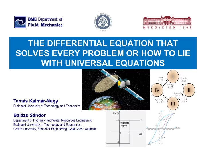
II I III IV

2 153

Miklós Farkas Seminar on Applied Analysis, 2018/02/15

SOLVING EVERY PROBLEM

3 153

Miklós Farkas Seminar on Applied Analysis, 2018/02/15

THANK YOU!

QUESTIONS?

4 153

Miklós Farkas Seminar on Applied Analysis, 2018/02/15

SOLVING EVERY PROBLEM

Theorem (Rubel, 1981) : There exists a fourth-

• rder Algebraic Differential Equation (ADE)

Py,y,y,y  0

that has a solution arbitrarily close to any smooth function for all t

Def: Let F be a class of real-valued functions defined on D⊆R. An ADE is called universal with respect to F(D), if every continuous function on F can be uniformly approximated by F-solutions of this ADE on D.

5 153

Miklós Farkas Seminar on Applied Analysis, 2018/02/15

CONSTRUCTING UNIVERSAL EQUATIONS

Universal Equation Recipe:

• 1. Take an ounce of sigmoid
• 2. Differentiate, then differentiate again
• 3. Eliminate constants
• 4. Shake, not stir

6 153

Miklós Farkas Seminar on Applied Analysis, 2018/02/15

• 1. TAKE AN OUNCE OF SIGMOID

finite sigmoid f on [0,1] f0  0, f1  1 f0  f1  0 ft  0, t  0,1. # # #

yt  Aft    B

The constants A, B, α, β serve to shift and scale the sigmoid

7 153

Miklós Farkas Seminar on Applied Analysis, 2018/02/15

WHY A SIGMOID?

f is a sigmoid on [0,1]

yt  Aft    B

Any continuous function can be arbitrarily approximated by concatenating scaled and shifted sigmoids

8 153

Miklós Farkas Seminar on Applied Analysis, 2018/02/15

• 2. DIFFERENTIATE, THEN DIFFERENTIATE AGAIN

yt  Aft  

yt  A2ft  ,  ynt  Anfnt  . #

The constant B can simply be eliminated by differentiating More constants? More differentiation…

9 153

Miklós Farkas Seminar on Applied Analysis, 2018/02/15

• 3. ELIMINATE CONSTANTS

Py,,yn  PAf,,Anfn  0

that are independent of the constants A and α. Look for equations of the form

gt  ft  

PAg,A2g,A3g,A4g,   0

Introduce the “kernel”

10 153

Miklós Farkas Seminar on Applied Analysis, 2018/02/15

• 4. SHAKE, NOT STIR (RUBEL’S EXAMPLE)

Assume a given form for the kernel

gt  e

1 t21

1  t  1

• therwise

3y4yy2  4y4y2y  6y3y2yy  24y2y4y  12y3yy3  29y2y3y2  12y7  0. #

PAg,A2g,A3g,A4g  0

Shake with some algebra

11 153

Miklós Farkas Seminar on Applied Analysis, 2018/02/15

OTHER UNIVERSAL EQUATIONS

2n2  3n  1y3  3n  1nyyy  n2y2y  0

Duffin 1981

gt  1  t2n

yy2  3yyy  21 

1 n y3  0 Briggs 2002

12 153

Miklós Farkas Seminar on Applied Analysis, 2018/02/15

CAN WE CONSTRUCT ALL UNIVERSAL EQUATIONS?

To "eliminate" the constants A and α we need P be a homogeneous polynomial of degree D

PAg,A2g,A3g,A4g,   AgDP  g

g ,2 g g ,3 g g ,

 0

Introduce the logarithmic derivative

ht 

gt gt

g  hg, g  hg  hg  h  h2g, g  h  3hh  h3g, g4  h  4hh  3h2  6h2h  h4g # # # #

Ph,2h  h2,3h  3hh  h3,4h  4hh  3h2  6h2h  h4,  



i

cib12b23b34b4hb1h  h2b2h  3hh  h3b3h  4hh  3h2  6h2h  h4b4 0. # #

b1  2b2  3b3  4b4  W

weight

13 153

Miklós Farkas Seminar on Applied Analysis, 2018/02/15

CONSTRUCTING UNIVERSAL EQUATIONS

The derivatives of h in terms of the derivatives of y

h  y y , h  yy  y2 y2 , h  2y3  3yyy  y2y y3 , h  6y4  12yy2y  3y2y2  4y2yy4  y3y5 y4 . #

h  h2  y y , h  3hh  h3  y4 y , h  4hh  3h2  6h2h  h4  y5 y ,



i b12b23b34b4W

ci

y y b1 y y b2 y4 y b3 y5 y b4 0

14 153

Miklós Farkas Seminar on Applied Analysis, 2018/02/15

CONSTRUCTING UNIVERSAL EQUATIONS

W  2

b1  2b2  2

b1 b2 W  bi 1 1 2



i,b12b2W

ciy

W biyb1yb2  c1yy  c2y2

The simplest Universal Differential Equation?

15 153

Miklós Farkas Seminar on Applied Analysis, 2018/02/15

CONSTRUCTING UNIVERSAL EQUATIONS

W  3

b1  2b2  3b3  3

b1 b2 b3 3 1 1 1 W  bi 1 2



i,b12b23b3W

ciy

W biyb1yb2yb3  c1y3  c2yyy  c3y2y

16 153

Miklós Farkas Seminar on Applied Analysis, 2018/02/15

CONSTRUCTING UNIVERSAL EQUATIONS

W  5

b1  2b2  3b3  4b4  5b5  5

b1 b2 b3 b4 b5 W  bi 5 3 1 1 1 2 2 2 1 2 1 1 3 1 1 3 1 4



i,b12b23b34b45b5W

ciy

W biyb1yb2yb3y5 b4y6 b5 

c1y5  c2yy3y  c3y2y2y4  c4y2yy2  c5y3yy5  c6y3yy4  c7y4y6 # #

WHAT ARE THE CORRESPONDING KERNELS/SIGMOIDS?

17 153

Miklós Farkas Seminar on Applied Analysis, 2018/02/15

ANOTHER DIRECTION: LIE GROUPS

The theory of Lie-groups contains powerful tools to analysing differential

• equations. It has been developed by

Marius Sophus Lie at the end of the XIX.-th century.

18 153

Miklós Farkas Seminar on Applied Analysis, 2018/02/15

LIE-POINT TRANSFORMATION GROUPS AS SYMMETRY GROUPS OF DIFFERENTIAL EQUATIONS

Let G be a Lie-group acting on the M manifold. Let M be locally the total space of the independent (m) and dependent (n) variables of a differential equation. G is a symmetry group of the differential equation if it transforms its solutions into another solutions on M. Example 1.: Let G be the one parameter group of the shifts of the independent variable (t) of an ODE (with y(t) as unknown). The group elements act on the (t,y) plane as:

= ≃ ℝ × ℝ ∗ = + ε, ∗ = → , , ε = + ε, , , ε = ∈ , , ∈ ≃ ℝ × ℝ

19 153

Miklós Farkas Seminar on Applied Analysis, 2018/02/15

AFFINE GROUP OF THE SOLUTION PLANE OF UNIVERSAL DIFFERENTIAL EQUATIONS

ft  Aft    B

To be universal, a differential equation must have a solution with which an arbitrary function can be uniformly approximated. Hence a universal differential equation must be form invariant under translations and scaling. Working definition An algebraic differential equation is universal if i.) it has a nonconstant solution whose derivatives vanish at the endpoints of a finite interval, ii.) it has the four parameter symmetry group of the affine transformations of the plane of the independent and dependent variable.

20 153

Miklós Farkas Seminar on Applied Analysis, 2018/02/15

AFFINE GROUP OF THE SOLUTION PLANE OF UNIVERSAL DIFFERENTIAL EQUATIONS

We introduce the affine group of the plane of the independent (t) and dependent variable (y) with its Lie algebra in operator form:

g  v1,v2,v3,v4

v1 

 t , v2  t  t , v3   y , v4  y  y

translation scaling The affine group of the plane is a symmetry group of the differential algebraic expression

Py,,yn : Rn  R

if it is invariant under the n-th extension (prolongation) of the infinitesimal generators

v1 nP  0, v2 nP  0, v3 nP  0, v4 nP  0

21 153

Miklós Farkas Seminar on Applied Analysis, 2018/02/15

AFFINE GROUP OF THE SOLUTION PLANE OF UNIVERSAL DIFFERENTIAL EQUATIONS

The n-th prolongation of the group action (with the infinitesimal operator representation ) describes how the derivatives of y ( ) behave under the group

• action. The invariance condition is stated in the n-th jet

space Jⁿ:(t, ) of the total space of the independent, and dependent variable (the (t,y) plane).

vn

yt ,ytt ,,yn

v  t,y 

t  t,y  y

vn   

t    y  1  yt  2  ytt    n  yn

1t,y,yt  Dt  ytDt, 2t,y,yt,ytt  Dt1  yttDt,  nt,y,yt,ytt,,yn  Dtn1  ynDt, #

Dt 

 t  yt  y  ytt  yt  

yt ,ytt ,,yn

22 153

Miklós Farkas Seminar on Applied Analysis, 2018/02/15

EXAMPLE: RUBEL’S EQUATION v1 n  v1 , v2 n  v2  yt  yt  2ytt  ytt    nyn  yn , v3 n  v3 , v4 n  v4  yt  yt  ytt  ytt    yn  yn . # PRubel  Py,y,y,y  3y4yy2  4y4y2y  6y3y2yy  24y2y4y  12y3yy3  29y2y3y2  12y7, #

v1 4 PRubel  0, v2 4 PRubel  0, v3 4 PRubel  0, v4 4 PRubel  0

23 153

Miklós Farkas Seminar on Applied Analysis, 2018/02/15

SOLVING EVERY PROBLEM

24 153

Miklós Farkas Seminar on Applied Analysis, 2018/02/15

THE MINIMAL UNIVERSAL EQUATION

The simplest universal equation

25 153

Miklós Farkas Seminar on Applied Analysis, 2018/02/15

FIRST INTEGRALS

First integrals are conserved quantities of the underlying dynamical system

• provides qualitative information about behavior
• can be used to reduce the order of the differential

equation

• useful in stability analysis
• can many times be related to the symmetries

Construction: many times ad hoc Here: an intuitive approach, backed by Lie methods

x   fx,x 

 : R2  R; x  x

First integral

26 153

Miklós Farkas Seminar on Applied Analysis, 2018/02/15

THE TOTAL DERIVATIVE

Integrating factor

27 153

Miklós Farkas Seminar on Applied Analysis, 2018/02/15

GEOMETRIC VIEW

28 153

Miklós Farkas Seminar on Applied Analysis, 2018/02/15

SECOND ORDER EQUATIONS

29 153

Miklós Farkas Seminar on Applied Analysis, 2018/02/15

USING LIE

Symmetry condition Parabolic PDE!

30 153

Miklós Farkas Seminar on Applied Analysis, 2018/02/15

EXAMPLES

31 153

Miklós Farkas Seminar on Applied Analysis, 2018/02/15

SYMMETRY EQUATION

32 153

Miklós Farkas Seminar on Applied Analysis, 2018/02/15

DAMPED OSCILLATOR

33 153

Miklós Farkas Seminar on Applied Analysis, 2018/02/15

NONLINEAR OSCILLATOR

34 153

Miklós Farkas Seminar on Applied Analysis, 2018/02/15

THANK YOU!

QUESTIONS?