The 2 k Factorial Design A design with k factors each with just 2 - PowerPoint PPT Presentation

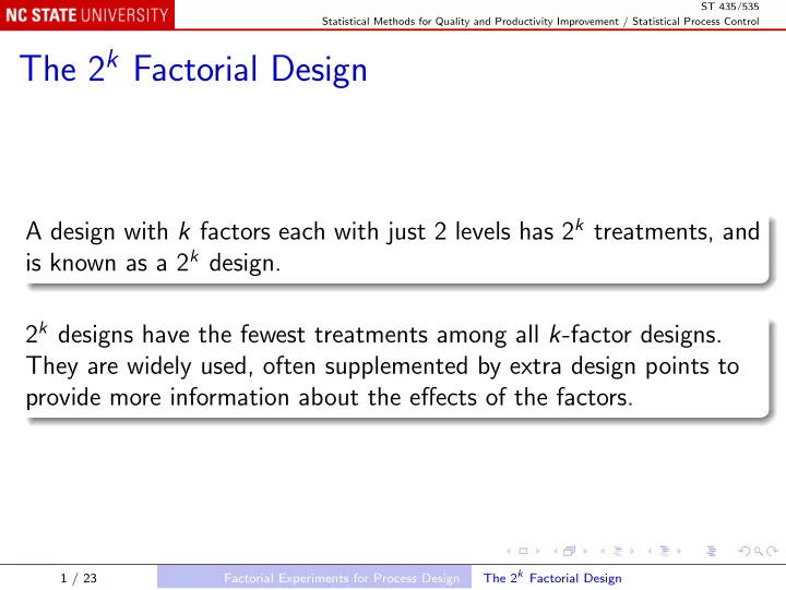
ST 435/535 Statistical Methods for Quality and Productivity Improvement / Statistical Process Control The 2 k Factorial Design A design with k factors each with just 2 levels has 2 k treatments, and is known as a 2 k design. 2 k designs have the fewest treatments among all k -factor designs. They are widely used, often supplemented by extra design points to provide more information about the effects of the factors. The 2 k Factorial Design 1 / 23 Factorial Experiments for Process Design

ST 435/535 Statistical Methods for Quality and Productivity Improvement / Statistical Process Control Example: The router experiment Problem: too much variability in dimensions of notches in PC boards. The experiment: vibration during cutting was used as an indicator of notch variability. Factors: 16 ” and 1 1 Bit size ( A ), with levels 8 ”; Speed ( B ), with levels 40 and 80 rpm. Replicated: n = 4 replications of each of the 2 2 = 4 treatments. The 2 k Factorial Design 2 / 23 Factorial Experiments for Process Design

ST 435/535 Statistical Methods for Quality and Productivity Improvement / Statistical Process Control In R: router <- read.csv("Data/Table-13-08.csv") summary(aov(Vibration ~ A * B, router)) Both factors have significant effects, and the interaction is also significant. The interaction plot: with(router, interaction.plot(A, B, Vibration)) Vibration is low when A (bit size) is at its low level, for either level of B (speed). The 2 k Factorial Design 3 / 23 Factorial Experiments for Process Design

ST 435/535 Statistical Methods for Quality and Productivity Improvement / Statistical Process Control Regression equation To predict what the vibration would be for other settings, we need a regression equation: E ( Y ) = β 0 + β 1 x 1 + β 2 x 2 + β 1 , 2 x 1 x 2 . It is convenient to use coded variables: � +1 if A is at its high level x 1 = − 1 if A is at its low level � +1 if B is at its high level x 2 = − 1 if B is at its low level The 2 k Factorial Design 4 / 23 Factorial Experiments for Process Design

ST 435/535 Statistical Methods for Quality and Productivity Improvement / Statistical Process Control router$x1 <- ifelse(router$A == "+", 1, -1) router$x2 <- ifelse(router$B == "+", 1, -1) summary(lm(Vibration ~ x1 * x2, router)) The fitted equation is y = 23 . 83 + 8 . 32 x 1 + 3 . 77 x 2 + 4 . 36 x 1 x 2 ˆ Note that the P -value associated with each coefficient is the same as the corresponding P -value in the analysis of variance table. The 2 k Factorial Design 5 / 23 Factorial Experiments for Process Design

ST 435/535 Statistical Methods for Quality and Productivity Improvement / Statistical Process Control The part of the data set involving x 1 and x 2 is: x 1 x 2 -1 -1 -1 -1 -1 -1 -1 -1 +1 -1 +1 -1 +1 -1 +1 -1 -1 +1 -1 +1 -1 +1 -1 +1 +1 +1 +1 +1 +1 +1 +1 +1 The 2 k Factorial Design 6 / 23 Factorial Experiments for Process Design

ST 435/535 Statistical Methods for Quality and Productivity Improvement / Statistical Process Control Add a column of 1’s and column for x 1 x 2 : 1 x 1 x 2 x 1 x 2 1 -1 -1 +1 1 -1 -1 +1 1 -1 -1 +1 1 -1 -1 +1 1 +1 -1 -1 1 +1 -1 -1 1 +1 -1 -1 1 +1 -1 -1 1 -1 +1 -1 1 -1 +1 -1 1 -1 +1 -1 1 -1 +1 -1 1 +1 +1 +1 1 +1 +1 +1 1 +1 +1 +1 1 +1 +1 +1 The 2 k Factorial Design 7 / 23 Factorial Experiments for Process Design

ST 435/535 Statistical Methods for Quality and Productivity Improvement / Statistical Process Control These four columns (divided by 16) are the coefficients needed to compute ˆ β 0 , ˆ β 1 , ˆ β 2 , and ˆ β 1 , 2 , respectively. The estimates could be calculated by hand using this table. We’ll use tables like this later to study the effects of blocking and to construct fractionally replicated designs. The 2 k Factorial Design 8 / 23 Factorial Experiments for Process Design

ST 435/535 Statistical Methods for Quality and Productivity Improvement / Statistical Process Control Physical variables The equation may be rewritten in terms of the physical variables x ∗ 1 = bit size, in inches x ∗ 2 = speed, in rpm router$bitsize <- ifelse(router$A == "+", 1/8, 1/16) router$speed <- ifelse(router$B == "+", 80, 40) summary(lm(Vibration ~ bitsize * speed, router)) The fitted equation is y = 26 . 78 − 152 x ∗ ˆ 1 − 0 . 465 x ∗ 2 + 6 . 97 x ∗ 1 x ∗ 2 . The 2 k Factorial Design 9 / 23 Factorial Experiments for Process Design

ST 435/535 Statistical Methods for Quality and Productivity Improvement / Statistical Process Control The equation in physical variables is more useful for predicting the response under new conditions of bit size and speed. However, its statistical interpretation is not as clear as when coded variables are used. Note that x ∗ 2 = 60 + 20 x 2 , and that x ∗ 1 is similarly a linear function of x 1 . These relationships can be used to transform the equation in x 1 and x 2 into the equation in x ∗ 1 and x ∗ 2 , without actually refitting the model. The 2 k Factorial Design 10 / 23 Factorial Experiments for Process Design

ST 435/535 Statistical Methods for Quality and Productivity Improvement / Statistical Process Control More general equations This regression equation is a special case of the general second-order model E ( Y ) = β 0 + β 1 x 1 + β 2 x 2 + β 1 , 2 x 1 x 2 + β 1 , 1 x 2 1 + β 2 , 2 x 2 2 with β 1 , 1 = β 2 , 2 = 0. This equation cannot be fitted to these data. Extra runs are needed, such as: Center points: x 1 = x 2 = 0; Axial points: x 1 = 0 , x 2 = ± α and x 2 = 0 , x 1 = ± α , where α could be 1, but is often larger. The 2 k Factorial Design 11 / 23 Factorial Experiments for Process Design

ST 435/535 Statistical Methods for Quality and Productivity Improvement / Statistical Process Control More than 2 factors The design and analysis of experiments with k > 2 two-level factors builds on the 2 2 case. The basic statistical model includes interaction terms for more than two factors at a time, which are difficult to interpret. In practice, it is often found that only a few factors are “active”, and that no high-order interactions are important. The 2 k Factorial Design 12 / 23 Factorial Experiments for Process Design

ST 435/535 Statistical Methods for Quality and Productivity Improvement / Statistical Process Control Example: Surface finish Response is the surface finish of a metal part. Factors, each with two levels: A : feed rate; B : depth of cut; C : tool angle. Two replications of each treatment. In R: finish <- read.csv("Data/Table-13-12.csv") summary(aov(Finish ~ A * B * C, finish)) The 2 k Factorial Design 13 / 23 Factorial Experiments for Process Design

ST 435/535 Statistical Methods for Quality and Productivity Improvement / Statistical Process Control Note that every line that involves C has a P -value greater than 0.18, so it appears that C has no effect, either overall or on the effects of A and B . If C is ignored, the design collapses (or projects ) onto a 2 × 2 design with 4 replicates. with(finish, interaction.plot(A, B, Finish)) The interaction plot shows that the finish is best (lowest) when A (feed rate) is at its low level, and then the level of B (depth of cut) is unimportant. The 2 k Factorial Design 14 / 23 Factorial Experiments for Process Design

ST 435/535 Statistical Methods for Quality and Productivity Improvement / Statistical Process Control Single replicate In the model with all interactions, the degrees of freedom for error are a × b × ... × ( n − 1), where n is the number of replications of each treatment. When n = 1, we have no estimate of σ 2 , so we cannot estimate the standard error of any parameter, and we cannot test hypotheses about the parameters or set up confidence intervals. Various procedures have been proposed to distinguish important effects from the rest. The simplest and most widely used is the half-normal plot of the estimated effects. The 2 k Factorial Design 15 / 23 Factorial Experiments for Process Design

ST 435/535 Statistical Methods for Quality and Productivity Improvement / Statistical Process Control Example: Plasma etching Four factors: Gap ( A ): spacing between anode and cathode; Pressure ( B ): in the etching vessel; Flow ( C ): flow rate of hexafluoroethane; Power ( D ): applied to the cathode. A single completely randomized run of the 2 4 design The 2 k Factorial Design 16 / 23 Factorial Experiments for Process Design

ST 435/535 Statistical Methods for Quality and Productivity Improvement / Statistical Process Control In R: plasma <- read.csv("Data/Table-13-15.csv") summary(aov(Rate ~ A * B * C * D, plasma)) library(gplots) qqnorm(aov(Rate ~ A * B * C * D, plasma), label = TRUE) No F -ratios or P -values are given. In the half-normal plot, A , D , and their interaction are the most prominent points. with(plasma, interaction.plot(A, D, Rate)) The 2 k Factorial Design 17 / 23 Factorial Experiments for Process Design