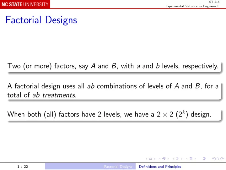
Factorial Designs Two (or more) factors, say A and B , with a and b - PowerPoint PPT Presentation

ST 516 Experimental Statistics for Engineers II Factorial Designs Two (or more) factors, say A and B , with a and b levels, respectively. A factorial design uses all ab combinations of levels of A and B , for a total of ab treatments . When both (all) factors have 2 levels, we have a 2 × 2 (2 k ) design. 1 / 22 Factorial Designs Definitions and Principles

ST 516 Experimental Statistics for Engineers II E.g. a 2 × 2 experiment: Factor A Low High Factor B High 30 52 Low 20 40 Main effect of A is Average response for high level of A − Average response for low level of A = 40 + 52 − 20 + 30 = 21 2 2 Similarly, main effect of B is 11. 2 / 22 Factorial Designs Definitions and Principles

ST 516 Experimental Statistics for Engineers II Interaction The simple effect of A at B − is 40 − 20 = 20, and the simple effect of A at B + is 52 − 30 = 22. The difference between these simple effects is the interaction AB (actually, one half the difference). Graphical presentation: the interaction plot. 3 / 22 Factorial Designs Definitions and Principles

ST 516 Experimental Statistics for Engineers II In R; lines are parallel if interaction is 0: twobytwo <- data.frame(A = c("-", "+", "-", "+"), B = c("+", "+", "-", "-"), y = c(30, 52, 20, 40)) interaction.plot(twobytwo$A, twobytwo$B, twobytwo$y) # or, saving some typing: with(twobytwo, interaction.plot(A, B, y)) 50 B + − mean of y 40 30 20 − + A 4 / 22 Factorial Designs Definitions and Principles

ST 516 Experimental Statistics for Engineers II The other way; lines are still parallel if interaction is 0: with(twobytwo, interaction.plot(B, A, y)) 50 A + − mean of y 40 30 20 − + B 5 / 22 Factorial Designs Definitions and Principles

ST 516 Experimental Statistics for Engineers II Interaction with Two Quantitative Factors Write the general level of factor A as x 1 , the general level of factor B as x 2 , and the response as y . Code x 1 so that x 1 = − 1 at A − and x 1 = +1 at A + , and x 2 similarly. Estimate the regression model representation y = β 0 + β 1 x 1 + β 2 x 2 + β 1 , 2 x 1 x 2 + ǫ. 6 / 22 Factorial Designs Definitions and Principles

ST 516 Experimental Statistics for Engineers II Least squares estimates of the β ’s can be found from the main effects and interaction. For the simple example: twobytwo$x1 <- ifelse (twobytwo$A == "+", 1, -1) twobytwo$x2 <- ifelse (twobytwo$B == "+", 1, -1) summary(lm(y ~ x1 * x2, twobytwo)) from which we get ˆ y = 35 . 5 + 10 . 5 x 1 + 5 . 5 x 2 + 0 . 5 x 1 x 2 . A graph of ˆ y versus x 1 and x 2 is called a response surface plot . 7 / 22 Factorial Designs Definitions and Principles

ST 516 Experimental Statistics for Engineers II 50 40 yhat 30 1.0 0.5 20 0.0 x2 −1.0 −0.5 −0.5 0.0 x1 0.5 −1.0 1.0 8 / 22 Factorial Designs Definitions and Principles

ST 516 Experimental Statistics for Engineers II Making the Response Surface Plot in R Use expand.grid() to set up a grid of values of x 1 and x 2 , use the predict() method to evaluate ˆ y on the grid, and use persp() to make a surface plot of it: ngrid <- 20 x1 <- with(twobytwo, seq(min(x1), max(x1), length = ngrid)) x2 <- with(twobytwo, seq(min(x2), max(x2), length = ngrid)) grid <- expand.grid(x1 = x1, x2 = x2) yhat <- predict(lm(y ~ x1 * x2, twobytwo), grid) yhat <- matrix(yhat, length(x1), length(x2)) persp(x1, x2, yhat, theta = 25, expand = 0.75, ticktype = "detailed") 9 / 22 Factorial Designs Definitions and Principles

ST 516 Experimental Statistics for Engineers II A Two-Factor Example Battery life data; A = Material, a = 3, B = Temperature, b = 3, replications n = 4 (battery-life.txt): Material Temperature Life 1 15 130 1 15 155 ... 1 125 20 ... 2 15 150 ... 2 125 45 3 15 138 ... 3 125 60 10 / 22 Factorial Designs Two-Factor Design

ST 516 Experimental Statistics for Engineers II boxplot(Life ~ factor(Material) * factor(Temperature), batteryLife) 150 100 50 1.15 2.15 3.15 1.70 2.70 3.70 1.125 2.125 3.125 11 / 22 Factorial Designs Two-Factor Design

ST 516 Experimental Statistics for Engineers II Statistical model y i , j , k = µ + τ i + β j + ( τβ ) i , j + ǫ i , j , k is the response for Material i , Temperature j , replicate k . τ ’s, β ’s, and ( τβ )’s satisfy the usual constraints (natural or computer). Hypotheses No differences among Materials; H 0 : τ i = 0, all i ; No effect of Temperature; H 0 : β j = 0, all j ; No interaction; H 0 : ( τβ ) i , j = 0, all i and j . 12 / 22 Factorial Designs Two-Factor Design

ST 516 Experimental Statistics for Engineers II R command batteryLife <- read.table("data/battery-life.txt", header = TRUE) summary(aov(Life ~ factor(Material) * factor(Temperature), batteryLife)) Output Df Sum Sq Mean Sq F value Pr(>F) factor(Material) 2 10684 5342 7.9114 0.001976 ** factor(Temperature) 2 39119 19559 28.9677 1.909e-07 *** factor(Material):factor(Temperature) 4 9614 2403 3.5595 0.018611 * Residuals 27 18231 675 --- Signif. codes: 0 *** 0.001 ** 0.01 * 0.05 . 0.1 1 13 / 22 Factorial Designs Two-Factor Design

ST 516 Experimental Statistics for Engineers II Interaction plots Can be made in two ways: Lifetime versus Temperature, with one curve for each type of Material; Lifetime versus Material, with one curve for each level of Temperature. Same information either way, but usually easier to interpret with a quantitative factor on the X-axis. Here Temperature is quantitative, but Material is qualitative . 14 / 22 Factorial Designs Two-Factor Design

ST 516 Experimental Statistics for Engineers II with(batteryLife, interaction.plot(Temperature, Material, Life, type = "b")) 160 2 Material 3 3 140 3 3 1 1 1 120 2 2 2 mean of Life 100 3 80 60 1 1 2 15 70 125 Temperature 15 / 22 Factorial Designs Two-Factor Design

ST 516 Experimental Statistics for Engineers II with(batteryLife, interaction.plot(Material, Temperature, Life, type = "b")) 160 1 Temperature 2 1 140 2 70 1 1 15 3 120 125 2 mean of Life 100 3 80 60 2 3 3 1 2 3 Material 16 / 22 Factorial Designs Two-Factor Design

ST 516 Experimental Statistics for Engineers II Pairwise comparisons TukeyHSD(aov(Life ~ factor(Material) * factor(Temperature), batteryLife)) Output Tukey multiple comparisons of means 95% family-wise confidence level Fit: aov(formula = Life ~ factor(Material) * factor(Temperature), data = batteryLife) $‘factor(Material)‘ diff lwr upr p adj 2-1 25.16667 -1.135677 51.46901 0.0627571 3-1 41.91667 15.614323 68.21901 0.0014162 3-2 16.75000 -9.552344 43.05234 0.2717815 $‘factor(Temperature)‘ diff lwr upr p adj 70-15 -37.25000 -63.55234 -10.94766 0.0043788 125-15 -80.66667 -106.96901 -54.36432 0.0000001 125-70 -43.41667 -69.71901 -17.11432 0.0009787 17 / 22 Factorial Designs Two-Factor Design

ST 516 Experimental Statistics for Engineers II $‘factor(Material):factor(Temperature)‘ diff lwr upr p adj 2:15-1:15 21.00 -40.823184 82.823184 0.9616404 3:15-1:15 9.25 -52.573184 71.073184 0.9998527 1:70-1:15 -77.50 -139.323184 -15.676816 0.0065212 2:70-1:15 -15.00 -76.823184 46.823184 0.9953182 3:70-1:15 11.00 -50.823184 72.823184 0.9994703 1:125-1:15 -77.25 -139.073184 -15.426816 0.0067471 2:125-1:15 -85.25 -147.073184 -23.426816 0.0022351 3:125-1:15 -49.25 -111.073184 12.573184 0.2016535 3:15-2:15 -11.75 -73.573184 50.073184 0.9991463 1:70-2:15 -98.50 -160.323184 -36.676816 0.0003449 2:70-2:15 -36.00 -97.823184 25.823184 0.5819453 3:70-2:15 -10.00 -71.823184 51.823184 0.9997369 1:125-2:15 -98.25 -160.073184 -36.426816 0.0003574 2:125-2:15 -106.25 -168.073184 -44.426816 0.0001152 3:125-2:15 -70.25 -132.073184 -8.426816 0.0172076 1:70-3:15 -86.75 -148.573184 -24.926816 0.0018119 2:70-3:15 -24.25 -86.073184 37.573184 0.9165175 ... 18 / 22 Factorial Designs Two-Factor Design

ST 516 Experimental Statistics for Engineers II Residual Plots plot(aov(Life ~ factor(Material) * factor(Temperature), batteryLife)); Residuals vs Fitted 4 ● 40 ● ● ● ● ● 20 ● ● ● ● ● ● ● ● ● Residuals ● ● ● 0 ● ● ● ● ● ● ● ● ● −20 ● ● ● ● ● ● ● −40 ● 9 −60 ● 3 60 80 100 120 140 160 Fitted values aov(Life ~ factor(Material) * factor(Temperature)) 19 / 22 Factorial Designs Two-Factor Design

ST 516 Experimental Statistics for Engineers II Normal Q−Q 2 4 ● ● ● Standardized residuals ● ● 1 ● ● ● ● ● ● ● ● ● ● ● ● ● ● 0 ● ● ● ● ● ● ● ● ● −1 ● ● ● ● ● ● 9 ● −2 ● 3 −2 −1 0 1 2 Theoretical Quantiles aov(Life ~ factor(Material) * factor(Temperature)) 20 / 22 Factorial Designs Two-Factor Design

ST 516 Experimental Statistics for Engineers II Scale−Location 3 ● 1.5 4 ● Standardized residuals ● 9 ● ● ● ● ● ● 1.0 ● ● ● ● ● ● ● ● ● ● ● ● ● ● ● ● ● 0.5 ● ● ● ● ● ● ● ● ● ● 0.0 60 80 100 120 140 160 Fitted values aov(Life ~ factor(Material) * factor(Temperature)) 21 / 22 Factorial Designs Two-Factor Design