= an orthogonal matrix T X X l l Cov( , ) i k ij kj j = - PowerPoint PPT Presentation

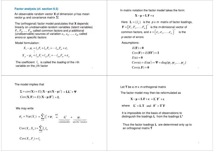
Factor analysis (cf. section 9.3) In matrix notation the factor model takes the form: An observable random vector X of dimension p has mean X LF − = + � ε vector � and covariance matrix Σ L Here is the p x m matrix of factor loadings, = l { } The (orthogonal) factor model postulates that X depends ij ′ [ ] F = is the m -dimisional vector of linearly on unobservable random variables (latent variables) F F … F , , , m 1 2 ′ F 1 , F 2 , ..., F m , called common factors and p additional =   ε ε ε  ε … , , , common factors, and is the  (unobservable) sources of variation ε 1 , ε 2 , ...., ε p , called p 1 2 p -vector of errors p -vector of errors errors or specific factors errors or specific factors Assumptions: Model formulation: F = 0 − µ = + + + ε E X l F l F ⋯ l F ( ) m m 1 1 11 1 12 2 1 1 ⋮ F FF ′ I = E = Cov( ) ( ) X − µ = l F + l F + l F + ε ⋯ 0 p p p p pm m p E = 1 1 2 2 ε ( ) The coefficient is called the loading of the i- th l ′ = = = ψ ψ ψ ε E εε Ψ … Cov( ) ( ) diag{ , , , } ij p 1 2 variable on the j -th factor ε F 0 Cov( , ) = 1 2 The model implies that Let T be a m x m orthogonal matrix = X = X − � X − ′ E LL ′ Σ � = + Ψ cov( ) {( )( ) } The factor model may then be reformulated as X F X � F ′ = E − = L Cov( , ) {( ) } X LF − = + = L F + � ε * * ε L LT F T F ′ = = * * where and We may write It is impossible on the basis of observations to It is impossible on the basis of observations to m m ∑ def σ = X = + ψ distinguish the loadings L from the loadings L* l 2 = + ψ Var( ) h 2 ii i ij i � � �� � � � �� � i i j = 1 communality specific variance Thus the factor loadings L are determined only up to m = ∑ an orthogonal matrix T X X l l Cov( , ) i k ij kj j = 1 = X F l Cov( , ) i j ij 4 3

We first consider estimation using principal components There are different methods for estimation of the Assume that Σ have eigenvalue-eigenvector pairs factor model λ e λ e λ e λ ≥ λ ≥ ≥ λ ≥ … ⋯ ( , ), ( , ), , ( , ) 0 where p p p 1 1 2 2 1 2 By the spectral decomposition we may write We will consider: e e ′ e e ′ e e ′ = λ + λ + + λ Σ ⋯ • estimation using principal components p p p 1 1 1 2 2 2 • maximum likelihood estimation • maximum likelihood estimation   e ′ λ  1 1  ⋯⋯⋯   e ′ For both methods the solution may be rotated by λ   2 2   = λ e λ e λ e ⋮ ⋮ ⋯ ⋮ multiplication by an orthogonal matrix to simplify the   ⋯⋯⋯    p p 1 1 2 2  ⋮ interpretation of factors (to be described later)   ⋯⋯⋯   e ′ λ   p p This is of the form with m = p and = LL ′ + 0 = Σ Ψ Ψ 5 6 The representation on the previous slide is not particularly Allowing for specific factors (errors) we obtain useful since we seek a representation with just a few common factors   e ′ λ   1 1 If the last p – m eigenvalues are small, we may neglect ⋯⋯⋯   e ′ λ e e ′ e e ′ λ + + λ ⋯ in the representation of Σ     2 2 ′ m + m + m + p p p ≈ LL + = λ e λ e λ e + ⋮ ⋮ ⋯ ⋮ 1 1 1 Σ Ψ Ψ      ⋯⋯⋯ m m 1 1 2 2    ⋮ ⋮     This gives: This gives: ⋯⋯⋯   λ e ′   e ′ λ    1 1  m m ⋯⋯⋯   ′ λ e     2 2 m ≈ λ e λ e λ e Σ ⋮ ⋮ ⋯ ⋮ − ∑   ⋯⋯⋯ = ψ ψ ψ ψ = σ    Ψ … l 2 diag{ , , , } m m where is given by 1 1 2 2 p i ii ij 1 2 ⋮  j = 1   ⋯⋯⋯   λ e ′   m m 7 8

The total sample variance is S s + s + + s = ⋯ tr( ) pp 11 22 The contribution to this from the j -th factor is ⌢ ɶ ɶ ɶ + + + = λ e ′ λ ˆ e = λ ˆ l l l 2 2 ⋯ 2 ( ) ( ) j j pj j j j j j 1 2 Thus contribution of total sample variance due to j -th factor is λ ˆ j + + + s s ⋯ s pp 11 22 (i.e. as for principal components) 9 10 How do we determine the number of factors? Example 9.3 (contd): In a consumer preference study a (if not given apriori) random sample of customers were asked to rate several attributes of a new product using a 7-point scale We want the m factors to explain as a fairly large proportion of the total sample variance, so may chose m so that this is achieved (subjectively) Sample correlation matrix For factor analysis of the correlation matrix R one may For factor analysis of the correlation matrix R one may let m be the number of eigenvalues larger than 1 One would also like the residual matrix ɶ ɶ ɶ S LL ′ − + Ψ ( ) to have small off-diagonal element (the diagonal elements are zero) 11 12

Example 9.4 The first two eigenvalues are the only ones larger than 1 and Weekly rates of return for five stocks on New York a model with two common factors accounts for 93% of the Stock Exchange Jan 2004 through Dec 2005 total (standardized) sample variance 13 14 We then consider estimation by maximum likelihood We now assume that the common factors F and the specific factors ε are multivariate normal Then X is multivariate normal with mean vector � ′ = LL + Σ Ψ and covariance matrix of the form Likelihood (based on n observations x 1 , x 2 , .... , x n ):   n 1 1 ∑ ′ = − x − − x − L � Σ  � Σ 1 �  ( , ) exp ( ) ( ) j j n π np / 2 / 2 Σ   (2 ) 2 = j 1 The likelihood may be maximized numerically L Ψ L ′ − 1 (under the condition that is a diagonal matrix) This gives the maximum likelihood estimates L Ψ ˆ ˆ = x � ˆ , (and ) 15 16

In general the correlation matrix ρ ρ  ⋯  The maximum likelihood estimates of the 1 p 12 1   ρ ρ communalities are ⋯ 1   ρ p =  21 2  ⋮ ⋮ ⋱ ⋮   ρ ρ ˆ = ˆ + ˆ + + ˆ = ⋯ h l l l i p   2 2 2 ⋯ 2 1   ( 1,...., ) p p 1 2 i i i im 1 2 ρ ρ = V = V − Σ V Σ V − 1/ 2 1/2 The contribution of the total sample variance due to The contribution of the total sample variance due to may be written as where may be written as where the j -th factor is   σ ⋯ 1 0 0  11  ˆ + ˆ + + ˆ l l l 2 2 ⋯ 2 σ   ⋯ 0 1 0 j j pj V − =  1 2 1/2 22  ⋮ ⋮ ⋱ ⋮ + + + s s ⋯ s   pp 11 22   σ ⋯ 0 0 1   pp is the inverse of the standard deviation matrix 17 18 LL ′ Example 9.5 = + Σ Ψ When we have that Weekly rates of return for five stocks on New York ρ = V − Σ V − 1/ 2 1/2 Stock Exchange Jan 2004 through Dec 2005 V LL ′ Ψ V = − + − 1/ 2 1/ 2 ( ) V − L V − L ′ V − Ψ V − = + 1/ 2 1/ 2 1/ 2 1/ 2 ( )( ) = L L ′ + Ψ z z z where L = V − L = V − Ψ V − 1/ 2 Ψ 1/ 2 1/ 2 and (diagonal) z z We obtain maximum likelihood estimates by inserting L V − 1/ 2 Ψ , and the maximum likelihood estimates for 19 20

Under the assumption that X is multivariate normal = LL ′ + Σ Ψ When one may show that the with mean vector � and covariance matrix Σ we maximum of the likelihood becomes may test the hypothesis that a factor model with m 1 = − np L e � Σ / 2 max ( , ) factors holds n / 2 � , Σ LL ′ = + Ψ π np ˆ / 2 Σ (2 ) This corresponds to test the null hypothesis ˆ ˆ ′ = LL ′ + ˆ = LL + ˆ H Σ Ψ Σ Ψ 0 : where − n / 2   ˆ Σ | | Λ =  Λ =  We may use the likelihood ratio test We may use the likelihood ratio test   The likelihood ratio takes the form The likelihood ratio takes the form S S  | |  n When we assume no structure on Σ the maximum of the For testing we may use that under H 0 likelihood becomes   ˆ Σ | | − Λ = n   1 2log log | = − np S L e � Σ / 2 max ( , ) |   n n S π np / 2 � , Σ / 2 (2 ) n is approximately chi-squared distributed with where S n = ( n -1) S / n p ( p +1)/2 – [ p ( m +1) – m ( m – 1)/2] degrees of freedom 21 22