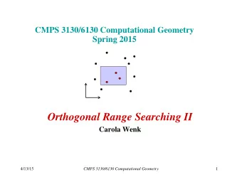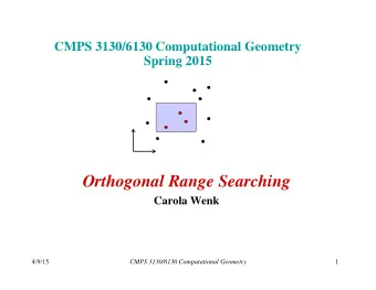
Orthogonal range searching Orthogonal range searching Problem: Given - PDF document

CG Lecture 4 CG Lecture 4 Orthogonal range searching Orthogonal range searching Problem: Given a set of n points Orthogonal range search in ℜ d , preprocess them such Y that reporting or counting the 1. Problem definition and motivation k points inside a d - dimensional axis-parallel box 2. Space decomposition: techniques and trade-offs (range) will be efficient. 3. Space decomposition schemes: X • Grids: uniform, non-hierarchical decomposition • Quad trees: uniform, hierarchical decomposition Sample application: Report all • Range trees and kd-trees: non-uniform, hierarchical cities within 20 KM radius of 4. Higher dimensions, variations on the theme Tel Aviv. 1 2 Space decomposition techniques Grids: uniform, non- -hierarchical hierarchical Space decomposition techniques Grids: uniform, non Method: • Different schemes for different types of data, with • Store points in a uniform array various trade-offs [1: n ]×[1: n ] • Types of space decomposition: • Query is answered by reporting • Grids : uniform, non-hierarchical decomposition points in subarray [ i : j ] ×[ k : l ] • Quad trees : uniform, hierarchical decomposition Complexity: • Range trees and kd-trees : non-uniform, hierarchical • Preprocessing in O ( n ) time and • Key efficiency parameters: O ( n 2 ) storage. Ω ( n ) • Preprocessing time: f ( n ) • Query time O ( k ). Ω ( n ) • Preprocessing storage f ( n ) • Update in O (1) when points on • Average query time f ( n,k ) grid. • Worst-case query time f ( n,k ) Alternatives: • Dynamical update (insertions/deletions) f ( n) 3 4 • List, sparse matrix, hashing Quad trees: construction Quad trees: construction Quad trees: uniform, hierarchical Quad trees: uniform, hierarchical Method : Method: • Start with smallest rectangle • Recursively partition the space containing all points. into four quadrants until leaf • Recusively classify point set into four quadrants contain a single point quadrants. or no point. • Stop when quadrant has one or no points. • Query is answered by recursively intersecting the query rectangle R The height h of the tree is related with the quadrants and reporting to the size of the initial rectangle s the results according to the and the smallest distance c between intersection. two points: h = log ( s / c ) + 3/2. i s/2 s/2 i Complexity : depends on the nature A quad tree with n points and of the data set, not just the height h has O ( h+1 ) n nodes and can be 5 6 number of points! constructed in O ( h+1 ) n time . 1

Quad trees: query answer Quad trees: query answer Non- Non -uniform, hierarchical decompositions uniform, hierarchical decompositions Method: Range tree At each evel, check how the query • Construct a binary search tree for coordinate x , and rectangle R intersects each quadrant: associate to each node in that tree a binary search • If it does not intersect, stop. tree for the y coordinate. • If it is included, report all points • Complexity: O ( n log n ) to build and store the trees, O (log 2 n +k ) to report k points. below • Else, recursively check each Kd-tree quadrant. • Construct a binary search tree by recursively Complexity: splitting the points along a median line alternating • Tests takes O (1) at each level. between in the x and y coordinates. • Worst case: must descend to deepest • Complexity: O ( n log n ) to build, O( n ) to store the tree, O ( √ n +k ) to report k points. level and test all four quadrants: O (4 ( h +1) ). 7 8 1D range searching 1D range searching Range searching in a 1D tree Range searching in a 1D tree • Find the two boundaries of the Points are real numbers, ranges are range in the leaves u and v . Input Range: 3.5-8.2 u defined by two numbers u and v . v • Report all leaves in maximal Algorithm: 1 1 sub-trees between u and v . -4 -2 0 1 3 5 7 11 • Sort points in O ( n log n ) time • Mark the vertex at which the v- -2 5 5 • Store points in a balanced binary search paths diverge as v-split . split 1 tree whose leaves are points. • Proceed to find the two -4 0 3 7 3 7 -2 5 boundaries, reporting values • Each tree node stores the in the sub-trees: largest value of its left subtree. -4 -2 0 1 7 11 3 5 5 7 11 - 4 0 3 7 When going to the left (right) • Do binary search for u and v endpoint of the range: If going left in the list in O(log n ) time. (right), report the entire right (left) -4 -2 0 1 3 5 7 11 subtree. When a leaf is reached, • List all values in between. check its value. Search complexity: O (log n + k ) Search complexity: 9 10 1D range query algorithm 1D range query algorithm 1D range trees – – split node finding split node finding 1D range trees 11 12 2

1D range query: run- -time analysis time analysis 2D range search: idea 1D range query: run 2D range search: idea Generalize 1D range searching: T T Construction: • k : output size • Construct a tree ordered by x T assoc ( v v ) ) T assoc ( • Leaves: O( k ) time coordinates. • Internal nodes: O( k ) time (since this is a v v • Each inner vertex v contains a binary tree) pointer to a secondary • Paths: O(log n ) time containing all the points of the primary subtree ordered • Total: O(log n + k ) time by y coordinate. • Worst case: k = n → Θ ( n ) time • Points are stored only in the sorted by y sorted by x secondary trees. 13 14 2D range tree: idea 2D range tree: idea 2D range tree construction algorithm 2D range tree construction algorithm Searching: T T • Given a 2D range, we simulate a 1D search and T assoc ( v v ) ) T assoc ( find subtrees sorted by x . v v • Instead of reporting the entire subtrees, invoke a search in the secondary trees sorted by y , and report only the points in the query range. 15 16 2D range tree construction complexity 2D range tree construction complexity 2D range tree construction complexity 2D range tree construction complexity • Same as a 1D-Tree, except that in each level the Improvement: secondary trees are built as well. • Source of inefficiency: repeated sorting by y • Theorem : The space complexity is Θ ( n log n ). coordinate! • Proof : The size of the primary tree is Θ ( n ). Each of its Θ (log n ) levels corresponds to a collection • Instead, sort by y only once , and copy data in the recursive calls in linear time. of secondary trees that contains all the n points. • Time complexity (naïve analysis): • The resulting recursive equation is: =  = O ( 1 ) n 1  O ( 1 ) n 1   =    T ( n ) n =    + T ( n ) n   O ( n ) 2 T else +    O ( n log n ) 2 T else     2    2 = O ( n log n ) 2 n = O ( n log ) 17 18 3

2D range tree query algorithm 2D range tree query algorithm 2D range search complexity 2D range search complexity Recurrence equation: ∑ = + + = + 2 T ( n ) O (log n ) (log n k ) O (log n k ) v v ↑ ↑ ↑ ↑ ↑ ↑ ↑ ↑ traversing traversing calls to traversing reporting calls to traversing reporting primary secondary primary secondary secondary secondary structure structure structure structure structure structure • The running time can be reduced to O (log n + k ) by using fractional cascading . 19 20 d- -dimensional range trees dimensional range trees d 2D kd kd trees: idea trees: idea 2D The idea generalizes directly to d • Bound the points by a rectangle. dimensions: T T • Split the points into two equal-size • Create a series of trees, one for subsets, using a horizontal or vertical each dimension. line. • Search each as before. v v • Continue recursively to partition the Complexity: subsets, alternating the directions of • Construction (time and storage) the lines, until point subsets are T d ( n ) = O ( n log n ) + T d–1 ( n ). O (log n ) small enough (of constant size). = O ( n log d–1 n ) • Canonical subsets are subtrees. • Query: sorted sorted sorted • In higher ( k ) dimensions: Split Q d ( n ) = O (log n ) + Q d–1 ( n ). O (log n ) by x 1 by x 2 by x 3 = O (log d n ) directions alternate between the k axes ( � kd trees). 21 22 2D kd kd tree construction tree construction 2D Example of a 2D kd Example of a 2D kd tree tree L 6 L 4 L 1 • Partition the plane into axis- G aligned rectangular regions. A E B L 3 • Nodes represent partition H L 2 F C lines, and leaves represent D input points. L 7 • The bottleneck is finding the L 5 median, which requires only L 1 linear time! • Time complexity: L 2 L 3  = O (1) n 1  =  T n ( )   L 4 L 5 L 6 L 7 n + > O n ( ) 2 T   n 1     2 23 24 = T n ( ) O n ( log ) n A B C D E F G H 4