Temporal Difference Methods, Off-Policy Methods Milan Straka - PowerPoint PPT Presentation
NPFL122, Lecture 3 Temporal Difference Methods, Off-Policy Methods Milan Straka October 21, 2019 Charles University in Prague Faculty of Mathematics and Physics Institute of Formal and Applied Linguistics unless otherwise stated Refresh
NPFL122, Lecture 3 Temporal Difference Methods, Off-Policy Methods Milan Straka October 21, 2019 Charles University in Prague Faculty of Mathematics and Physics Institute of Formal and Applied Linguistics unless otherwise stated
Refresh – Policies and Value Functions π ( a ∣ s ) π A policy computes a distribution of actions in a given state, i.e., corresponds to a a s probability of performing an action in state . ( s ) v π To evaluate a quality of a policy, we define value function , or state-value function , as def E ∞ ∣ π [∑ ] E ( s ) = π [ t ∣ = s = ] k = s . ∣ v G S γ R S t + k +1 ∣ π t t k =0 π An action-value function for a policy is defined analogously as def E ∞ ∣ π [∑ ] E k ( s , a ) = π [ t ∣ = s , A = a = ] = s , A = a . ∣ q G S γ R S t + k +1 ∣ π t t t t k =0 def max ( s ) = ( s ), v v ∗ π π def max Optimal state-value function is defined as analogously optimal action- ( s , a ) = ( s , a ). q q ∗ π π value function is defined as = π v v ∗ ∗ π ∗ Any policy with is called an optimal policy . NPFL122, Lecture 3 Refresh Monte Carlo Methods TD Q-learning Double Q Off-policy Expected Sarsa 2/34
Refresh – Value Iteration Optimal value function can be computed by repetitive application of Bellman optimality equation: ( s ) ← 0 v 0 E R ( s ) ← max [ + γv ( S t +1 ∣ ) S = s , A = a = Bv ] . v k +1 t +1 k t t k a γ < 1 Converges for finite-horizont tasks or when discount factor . NPFL122, Lecture 3 Refresh Monte Carlo Methods TD Q-learning Double Q Off-policy Expected Sarsa 3/34
Refresh – Policy Iteration Algorithm Policy iteration consists of repeatedly performing policy evaluation and policy improvement: E I E I E I I E 0 ⟶ 0 ⟶ 1 ⟶ 1 ⟶ 2 ⟶ 2 ⟶ … ⟶ ∗ ⟶ . π v π v π v π v π π π π ∗ ′ π = π π i The result is a sequence of monotonically improving policies . Note that when , also = v v v π π ′ π π , which means Bellman optimality equation is fulfilled and both and are optimal. Considering that there is only a finite number of policies, the optimal policy and optimal value function can be computed in finite time (contrary to value iteration, where the convergence is only asymptotic). π v k +1 π k Note that when evaluating policy , we usually start with , which is assumed to be a v π k +1 good approximation to . NPFL122, Lecture 3 Refresh Monte Carlo Methods TD Q-learning Double Q Off-policy Expected Sarsa 4/34
Refresh – Generalized Policy Iteration Generalized Policy Evaluation is a general idea of interleaving policy evaluation and policy improvement at various granularity. Figure in Section 4.6 of "Reinforcement Learning: An Introduction, Second Edition". Figure in Section 4.6 of "Reinforcement Learning: An Introduction, Second Edition". If both processes stabilize, we know we have obtained optimal policy. NPFL122, Lecture 3 Refresh Monte Carlo Methods TD Q-learning Double Q Off-policy Expected Sarsa 5/34
Monte Carlo Methods We now present the first algorithm for computing optimal policies without assuming a knowledge of the environment dynamics. S However, we still assume there are finitely many states and we will store estimates for each of them. Monte Carlo methods are based on estimating returns from complete episodes. Furthermore, if the model (of the environment) is not known, we need to estimate returns for the action-value q v function instead of . We can formulate Monte Carlo methods in the generalized policy improvement framework. Keeping estimated returns for the action-value function, we perform policy evaluation by sampling one episode according to current policy. We then update the action-value function by averaging over the observed returns, including the currently sampled episode. NPFL122, Lecture 3 Refresh Monte Carlo Methods TD Q-learning Double Q Off-policy Expected Sarsa 6/34
Monte Carlo Methods To guarantee convergence, we need to visit each state infinitely many times. One of the simplest way to achieve that is to assume exploring starts , where we randomly select the first state and first action, each pair with nonzero probability. Furthermore, if a state-action pair appears multiple times in one episode, the sampled returns are not independent. The literature distinguishes two cases: first visit : only the first occurence of a state-action pair in an episode is considered every visit : all occurences of a state-action pair are considered. Even though first-visit is easier to analyze, it can be proven that for both approaches, policy evaluation converges. Contrary to the Reinforcement Learning: An Introduction book, which presents first-visit algorithms, we use every-visit. NPFL122, Lecture 3 Refresh Monte Carlo Methods TD Q-learning Double Q Off-policy Expected Sarsa 7/34
Monte Carlo with Exploring Starts Modification of algorithm 5.3 of "Reinforcement Learning: An Introduction, Second Edition" from first-visit to every-visit. NPFL122, Lecture 3 Refresh Monte Carlo Methods TD Q-learning Double Q Off-policy Expected Sarsa 8/34
ε Monte Carlo and -soft Policies ε A policy is called -soft, if ε π ( a ∣ s ) ≥ . ∣ A ( s )∣ ε For -soft policy, Monte Carlo policy evaluation also converges, without the need of exploring starts. ε 1 − ε + ∣ A ( s )∣ ε We call a policy -greedy, if one action has maximum probability of . ε The policy improvement theorem can be proved also for the class of -soft policies, and using ε -greedy policy in policy improvement step, policy iteration has the same convergence ε properties. (We can embed the -soft behaviour “ inside ” the environment and prove equivalence.) NPFL122, Lecture 3 Refresh Monte Carlo Methods TD Q-learning Double Q Off-policy Expected Sarsa 9/34
ε Monte Carlo for -soft Policies ε On-policy every-visit Monte Carlo for -soft Policies ε > 0 Algorithm parameter: small Q ( s , a ) ∈ R s ∈ S , a ∈ A Initialize arbitrarily (usually to 0), for all C ( s , a ) ∈ Z s ∈ S , a ∈ A Initialize to 0, for all Repeat forever (for each episode): , A , R , … , S , A , R S 0 0 1 T −1 T −1 T Generate an episode , by generating actions as follows: ε def arg max With probability , generate a random uniform action t = Q ( S , a ) A t a Otherwise, set G ← 0 t = T − 1, T − 2, … , 0 For each : G ← γG + R T +1 C ( S , A ) ← C ( S , A ) + 1 t t t t 1 Q ( S , A ) ← Q ( S , A ) + ( G − Q ( S , A )) t t t t t t C ( S , A ) t t NPFL122, Lecture 3 Refresh Monte Carlo Methods TD Q-learning Double Q Off-policy Expected Sarsa 10/34
Action-values and Afterstates q The reason we estimate action-value function is that the policy is defined as def π ( s ) = arg max ( s , a ) q π a arg max ∑ ′ ] ′ = p ( s , r ∣ s , a ) r + γv [ ( s ) π ′ s , r a and the latter form might be impossible to evaluate if we do not have the model of the environment. However, if the environment is known, it might be better to estimate returns only for states, and there can be substantially less states than state-action pairs. Figure from section 6.8 of "Reinforcement Learning: An Introduction, Second Edition". NPFL122, Lecture 3 Refresh Monte Carlo Methods TD Q-learning Double Q Off-policy Expected Sarsa 11/34
Partially Observable MDPs ( S , A , p , γ ) Recall that a Markov decision process (MDP) is a quadruple , where: S is a set of states, A is a set of actions, ′ p ( S = s , R = r ∣ S = s , A = a ) a ∈ A t +1 t +1 t t is a probability that action will lead from r ∈ R ′ s ∈ S s ∈ S state to , producing a reward , γ ∈ [0, 1] is a discount factor . Partially observable Markov decision process extends the Markov decision process to a sextuple ( S , A , p , γ , O , o ) , where in addition to an MDP O is a set of observations, o ( O ∣ S , A ) t −1 t t is an observation model. Although planning in general POMDP is undecidable, several approaches are used to handle POMDPs in robotics (to model uncertainty, imprecise mechanisms and inaccurate sensors, … ). In deep RL, partially observable MDPs are usually handled using recurrent networks, which S t model the latent states . NPFL122, Lecture 3 Refresh Monte Carlo Methods TD Q-learning Double Q Off-policy Expected Sarsa 12/34
TD Methods Temporal-difference methods estimate action-value returns using one iteration of Bellman equation instead of complete episode return. α Compared to Monte Carlo method with constant learning rate , which performs v ( S ) ← v ( S ) + [ − v ( S t ] ) , α G t t t the simplest temporal-difference method computes the following: v ( S ) ← v ( S ) + [ + γv ( S ) − v ( S t ] ) , α R t +1 t +1 t t NPFL122, Lecture 3 Refresh Monte Carlo Methods TD Q-learning Double Q Off-policy Expected Sarsa 13/34
Recommend
More recommend
Explore More Topics
Stay informed with curated content and fresh updates.
