Bonus Lecture: Introduction to Reinforcement Learning Garima - PowerPoint PPT Presentation
Bonus Lecture: Introduction to Reinforcement Learning Garima Lalwani, Karan Ganju and Unnat Jain Credits: These slides and images are borrowed from slides by David Silver and Peter Abbeel 4 Model-free Control 5 Summary Outline 1 RL Problem
Bonus Lecture: Introduction to Reinforcement Learning Garima Lalwani, Karan Ganju and Unnat Jain Credits: These slides and images are borrowed from slides by David Silver and Peter Abbeel
4 Model-free Control 5 Summary Outline 1 RL Problem Formulation 2 Model-based Prediction and Control 3 Model-free Prediction
Part 1: RL Problem Formulation
Characteristics of Reinforcement Learning What makes reinforcement learning different from other machine learning paradigms? There is no supervisor, only a reward signal Feedback is delayed, not instantaneous Time really matters ( correlated , non i.i.d data) Agent’s actions affect the subsequent data it receives
Environment Agent Agent and Environment Observed state action S t A t reward R t
Rewards A reward R t is a scalar feedback signal Indicates how well agent is doing at step t The agent’s job is to maximise cumulative reward
Rod Balancing Demo https://www.youtube.com/watch?v=Lt-KLtkDlh8 Learn to swing up and balance a real pole based on raw visual input data, ICNIP 2012
RL based visual control End-to-end training of deep visuomotor policies, JMLR 2016 https://www.youtube.com/watch?v=CE6fBDHPbP8
RL based visual control Link: https://goo.gl/kY4RmS Source: https://68.media.tumblr.com/
https://deepmind.com/research/alphago/ Stanford autonomous helicopter Abbeel et. Al. https://gym.openai.com/ Examples of Rewards Fly stunt manoeuvres in a helicopter +ve reward for following desired trajectory − ve reward for crashing Play many Atari games better than humans + / − ve reward for increasing/decreasing score Defeat the world champion at Go + / − ve reward for winning/losing a game
Sample model of RL problem Home OH Arun's Disc. Group Complete Murphy's Project Pubbing R = -1 Submit Leave Pubbing project R = 0 R = 0 R = 0 R = -1 Submit project Study Study R = +10 R = -2 R = -2 R = -2 Take Arun's Quiz R = +1 0.4 0.2 0.4
States Home OH Arun's Disc. Group Complete Murphy's Project Pubbing R = -1 Submit Leave Pubbing project R = 0 R = 0 R = 0 R = -1 Submit project Study Study R = +10 R = -2 R = -2 R = -2 Take Arun's Quiz R = +1 0.4 0.2 0.4
Actions Home OH Arun's Disc. Group Complete Murphy's Project Pubbing R = -1 Submit Leave Pubbing project R = 0 R = 0 R = 0 R = -1 Submit project Study Study R = +10 R = -2 R = -2 R = -2 Take Arun's Quiz R = +1 0.4 0.2 0.4
Rewards Home Murphy's Project Complete Group Disc. Arun's OH Pubbing R = -1 R = -1 Submit Leave Pubbing project R = 0 R = 0 R = 0 R = 0 R = -1 R = -1 Submit project Study Study R = +10 R = +10 R = -2 R = -2 R = -2 R = -2 Take Arun's Quiz R = +1 R = +1 0.4 0.2 0.4
Transition probabilities Home OH Arun's Disc. Group Complete Murphy's Project Pubbing R = -1 Submit Leave Pubbing project R = 0 R = 0 R = -1 Submit project Study Study R = +10 R = -2 R = -2 Take Arun's Quiz R = +1 0.2 0.4 0.4 0.2 0.4 0.4
MDP Markov Decision Process A Markov decision process (MDP) is an environment in which all states are Markov Markov. P [ S t +1 | S t , A t = a ] = P [ S t +1 | S 1 , ..., S t , A t = a ] A Markov D ecision Process has the following �S , A , P , R , γ � S is a finite set of states A is a finite set of actions P is a state transition probability matrix, P a ′ ss ′ = P [ S t +1 = s | S t = s , A t = a ] a R is a reward function, R s = E [ R t +1 | S t = s , A t = a ]
Policy: agent’s behaviour function An RL agent may include one or more of these components: Model: agent’s representation of the environment Value function: how good is each state and/or action Major Components of an RL Agent
Policy A policy is the agent’s behaviour It is a map from state to action, e.g. Deterministic policy: π ( s ) = 1 for A t = a Stochastic policy: π ( a | s ) = P [ A t = a | S t = s ]
Actions Home OH Arun's Disc. Group Complete Murphy's Project Pubbing R = -1 Submit Leave Pubbing project R = 0 R = 0 R = 0 R = -1 Submit project Study Study R = +10 R = -2 R = -2 R = -2 Take Arun's Quiz R = +1 0.4 0.2 0.4
Model A model predicts what the environment will do next P : Transition probabilities R : Expected rewards ss ′ = P [ S t +1 = s ′ | S t = s , A t = a ] P a R a s = E [ R t +1 | S t = s , A t = a ]
Beyond Rewards Home OH Arun's Disc. Group Complete Murphy's Project Pubbing R = -1 Submit Leave Pubbing project R = 0 R = 0 R = 0 R = -1 Submit project Study Study R = +10 R = -2 R = -2 R = -2 Take Arun's Quiz R = +1 0.4 0.2 0.4
Value function - Concept of Return Return G t This values immediate reward above delayed reward. Avoids infinite returns in cyclic Markov processes The return G t is cumulative discounted discounted reward from time-step t . ∞ � γ k R t + k +1 G t = R t +1 + γ R t +2 + ... = k =0 The discount γ ∈ [0 , 1] is the present value of future rewards
State Value Function v π (s) Action Value Function q π (s,a) Value Function v π ( s ) = E π [ G t | S t = s ] v π ( s ) of an MDP is the expected return starting from state s , and then following policy π q π ( s , a ) = E π [ G t | S t = s , A t = a ] q π ( s , a ) is the expected return starting from state s , taking action a , and then following policy π
Subproblems in RL Model based Model free Prediction: evaluate the future Given a policy Control: optimise the future Find the best policy
Part 2: Model-based Prediction and Control
Connecting v(s) and q(s,a): Bellman equations q in terms of v : v in terms of q : v π ( s ) 7! s � v π ( s ) = π ( a | s ) q π ( s , a ) π ( a | s ) q π ( s , a ) a ∈A q π ( s, a ) 7! a π ( a 1 | s ) q π ( s , a ) π ( a n | s ) q π ( s , a ) q π ( s, a ) 7! s, a a + γ P a ss ′ v π ( s ′ ) � P a ss ′ v π ( s ′ ) q π ( s , a ) = R s r s ′ ∈S v π ( s 0 ) s 0 7!
Connecting v(s) and q(s,a): Bellman equations (2) q in terms of other q : v in terms of other v : v π ( s ) 7! s � � ss ′ v π ( s ′ ) a � � a v π ( s ) = π ( a | s ) R s + γ P a a ∈A s ′ ∈S r v π ( s 0 ) 7! s 0 q π ( s, a ) 7! s, a r q π ( s , a ) = R a � P a � s + γ π ( a ′ | s ′ ) q π ( s ′ , a ′ ) ss ′ s 0 s ′ ∈S a ′ ∈A q π ( s 0 , a 0 ) a 0 7!
Example: v π (s) Group Disc. Pubbing R = -1 -2.3 -2.3 0 Submit Leave Pubbing project R = 0 R = 0 R = -1 Submit project Study Study R = +10 -1.3 -1.3 7.4 7.4 R = -2 R = -2 Take Arun's Quiz R = +1 0.4 0.2 0.4
Example: v π (s) Group Disc. v π (s) for π (a|s)=0.5, γ =1 Pubbing v π (GD) = 0.5* (R+ v π (Submitted) ) + 0.5*(R+ v π (Arun's OH)) R = -1 v π (GD) = 0.5*(0+0) + 0.5*(-2 + 7.4) -2.3 -2.3 0 Submit Leave Pubbing project R = 0 R = 0 R = -1 Submit project Study Study R = +10 -1.3 -1.3 7.4 7.4 R = -2 R = -2 Take Arun's Quiz R = +1 0.4 0.2 0.4
Example: v π (s) v π (s) for π (a|s)=0.5, γ =1 Pubbing v π (GD) = 0.5* (R+ v π (Submitted) ) + 0.5*(R+ v π (Arun's OH)) R = -1 v π (GD) = 0.5*(0+0) + 0.5*(-2 + 7.4) -2.3 -2.3 0 Submit Leave Pubbing project R = 0 R = 0 R = -1 Submit project Study Study R = +10 -1.3 -1.3 2.7 2.7 7.4 7.4 R = -2 R = -2 Take Arun's Quiz R = +1 0.4 0.2 0.4
Example: q π (s,a) q π (s ,a ) for π (a|s)=0.5, γ =1 R = -1 q = - 3.3 q = 0 q = - 3.3 R = 0 R = -1 R = 0 q = 10 q = - 1.3 R = +10 q = 0.7 q = 5.4 R = -2 R = -2 q = 3.78 R = +1 0.4 0.2 0.4
Example: q π (s,a) q π (s ,a ) for π (a|s)=0.5, γ =1 R = -1 q = - 3.3 q = 0 q = - 3.3 R = 0 R = -1 R = 0 q = - 1.3 q = 10 R = +10 q = 0.7 q = 5.4 R = -2 R = -2 q = 3.78 R = +1 0.4 0.2 0.4
Example: Policy improvement R = -1 q = - 3.3 q = 0 q = - 3.3 R = 0 R = -1 R = 0 q = 10 q = - 1.3 R = +10 q = 0.7 q = 5.4 R = -2 R = -2 q = 3.78 R = +1 0.4 0.2 0.4
Example: Policy improvement - Greedy � 1 if a = argmax q old ( s , a ) R = -1 π new ( a | s ) = a ∈A q = - 3.3 0 otherwise q = 0 q = - 3.3 R = 0 R = -1 R = 0 q = 10 q = - 1.3 R = +10 q = 0.7 q = 5.4 R = -2 R = -2 q = 3.78 R = +1 0.4 0.2 0.4
Policy Iteration Policy evaluation Estimate v π Iterative policy evaluation Policy improvement Generate π ′ ≥ π Greedy policy improvement
Rewards: -1 for time step States: 14 cells + 2 terminal cells Actions: 4 directions Iterative Policy Evaluation in Small Gridworld V k for the Greedy Policy update v k w.r.t. V k Random Policy v k 0.0 0.0 0.0 0.0 0.0 0.0 0.0 0.0 random k = 0 policy 0.0 0.0 0.0 0.0 0.0 0.0 0.0 0.0 0.0 -1.0 -1.0 -1.0 -1.0 -1.0 -1.0 -1.0 k = 1 -1.0 -1.0 -1.0 -1.0 -1.0 -1.0 -1.0 0.0 -1.7 -2.0 -2.0 0.0 -1.7 -2.0 -2.0 -2.0 k = 2 -2.0 -2.0 -2.0 -1.7 -2.0 -2.0 -1.7 0.0 -2.4 -2.9 -3.0 0.0 -2.4 -2.9 -3.0 -2.9 = 3 -2.9 -3.0 -2.9 -2.4 -3.0 -2.9 -2.4 0.0 0.0 -6.1 -8.4 -9.0 optimal -6.1 -7.7 -8.4 -8.4 = 10 policy -8.4 -8.4 -7.7 -6.1 -9.0 -8.4 -6.1 0.0 0.0 -14. -20. -22. -14. -18. -20. -20. = -20. -20. -18. -14. -22. -20. -14. 0.0
Recommend
More recommend
Explore More Topics
Stay informed with curated content and fresh updates.
![Bonus * Bonus * Bonus * Bonus * Bonus * Bonus Bonus * Bonus * Bonus * Bonus * Bonus * Bonus + ]](https://c.sambuz.com/705281/bonus-bonus-bonus-bonus-bonus-bonus-bonus-bonus-bonus-s.webp)

