Synchronous Control and State Machines in Modelica Hilding Elmqvist - PowerPoint PPT Presentation
Synchronous Control and State Machines in Modelica Hilding Elmqvist Dassault Systmes Sven Erik Mattsson, Fabien Gaucher, Francois Dupont Dassault Systmes Martin Otter, Bernhard Thiele DLR Content Introduction Synchronous
Synchronous Control and State Machines in Modelica Hilding Elmqvist Dassault Systèmes Sven Erik Mattsson, Fabien Gaucher, Francois Dupont Dassault Systèmes Martin Otter, Bernhard Thiele DLR
Content • Introduction • Synchronous Features of Modelica • Synchronous Operators • Base-clock and Sub-clock Partitioning • Modelica_Synchronous library • State Machines • Conclusions Slide 2
Introduction • Why synchronous features in Modelica 3.3? model Asynchronous_Modelica33 model Asynchronous_Modelica32 Real x(start=0,fixed=true), Real x(start=0,fixed=true), y(start=0,fixed=true), z; y(start=0,fixed=true), z; equation equation when Clock(0.33) then when sample(0,0.33) then x = previous(x)+1; x = pre(x)+1; Rational number 1/3 end when; end when; when Clock(1,3) then when sample(0,1/3) then y = previous(y)+1; y = pre(y)+1; x and y must have end when; end when; Implicit hold the same clock z = x-y; z = x-y; end Asynchronous_Modelica33; end Asynchronous_Modelica32; z = x-y • Error Diagnostics for safer systems! Slide 3
Introduction • Scope of Modelica extended • Covers complete system descriptions including controllers • Clocked semantics • Clock associated with variable type and inferred • For increased correctness • Based on ideas from Lucid Synchrone and other synchronous languages • Extended with multi-rate periodic clocks, varying interval clocks and Boolean clocks Slide 4
Synchronous Features of Modelica • Plant and Controller Partitioning • Boundaries between continuous-time and discrete-time equations defined by operators. • sample(): samples a continuous-time variable and returns a clocked discrete-time expression • hold(): converts from clocked discrete-time to continuous-time by holding the value between clock ticks • sample operator may take a Clock argument to define when sampling should occur Slide 5
Mass with Spring Damper • Consider a continuous-time model partial model MassWithSpringDamper parameter Modelica.SIunits.Mass m=1; parameter Modelica.SIunits.TranslationalSpringConstant k=1; parameter Modelica.SIunits.TranslationalDampingConstant d=0.1; Modelica.SIunits.Position x(start=1,fixed=true) "Position"; Modelica.SIunits.Velocity v(start=0,fixed=true) "Velocity"; Modelica.SIunits.Force f "Force"; equation der(x) = v; m*der(v) = f - k*x - d*v; end MassWithSpringDamper; Slide 6
Synchronous Controller • Discrete-time controller model SpeedControl extends MassWithSpringDamper; parameter Real K = 20 "Gain of speed P controller"; parameter Modelica.SIunits.Velocity vref = 100 "Speed ref."; discrete Real vd; discrete Real u(start=0); Sample continuous velocity v equation with periodic Clock with period=0.01 // speed sensor vd = sample(v, Clock(0.01)); The clock of the equation // P controller for speed is inferred to be the same as for the variable u = K*(vref-vd); vd which is the result of sample() // force actuator Hold discrete variable u f = hold(u); between clock ticks end SpeedControl; Slide 7
Discrete-time State Variables • Operator previous() is used to access the value at the previous clock tick (cf pre() in Modelica 3.2) • Introduces discrete state variable • Initial value needed • interval() is used to inquire the actual interval of a clock Slide 8
Base-clocks and Sub-clocks • A Modelica model will typically have several controllers for different parts of the plant. • Such controllers might not need synchronization and can have different base clocks . • Equations belonging to different base clocks can be implemented by asynchronous tasks of the used operating system. • It is also possible to introduce sub-clocks that tick a certain factor slower than the base clock. • Such sub-clocks are perfectly synchronized with the base clock, i.e. the definitions and uses of a variable are sorted in such a way that when sub- clocks are activated at the same clock tick, then the definition is evaluated before all the uses. • New base type, Clock: Clock cControl = Clock(0.01); Clock cOuter = subSample(cControl, 5); Slide 9
Sub and super sampling and phase model SynchronousOperators Real u; Real sub; Real super; Real shift(start=0.5); Real back; equation u = sample(time, Clock(0.1)); sub = subSample(u, 4); super = superSample(sub, 2); shift = shiftSample(u, 2, 3); back = backSample(shift, 1, 3); end SynchronousOperators; Slide 10
Exact Periodic Clocks • Clocks defined by Real number period are not synchronized: Clock c1 = Clock(0.1); Clock c2 = superSample(c1,3); Clock c3 = Clock(0.1/3); // Not synchronized with c2 • Clocks defined by rational number period are synchronized: Clock c1 = Clock(1,10); // period = 1/10 Clock c2 = superSample(c1,3); // period = 1/30 Clock c3 = Clock(1,30); // period = 1/30 Slide 11
Modelica_Synchronous library • Synchronous language elements of Modelica 3.3 are “low level”: // speed sensor vd = sample(v, Clock(0.01)); // P controller for speed u = K*(vref-vd); // force actuator f = hold(u); • Modelica_Synchronous library developed to access language elements in a convenient way graphically: Slide 12
Blocks that generate clock signals Generates a periodic clock with a Real period parameter Modelica.SIunits.Time period; ClockOutput y; equation y = Clock(period); Generates a periodic clock as an integer multiple of a resolution (defined by an enumeration). Code for 20 ms period: y = superSample(Clock(20), 1000); super-sample clock with 1000 Clock with period 20 s period = 20 / 1000 = 20 ms Generates an event clock: The clock ticks whenever the continuous-time Boolean input changes from false to true. y = Clock(u); Slide 13
Sample and Hold Holds a clocked signal and generates a continuous-time signal. Before the first clock tick, the continuous-time output Discrete-time PI controller y is set to parameter y_start y = hold(u); Purely algebraic block from Samples a continuous-time signal Modelica.Blocks.Math and generates a clocked signal. y = sample(u); y = sample(u, clock); Slide 14
Sub- and Super-Sampling Defines that the output signal is an integer factor faster as the input signal, using a “hold” semantics for the signal. By default, this factor is inferred. It can also be defined explicitly. y = superSample(u); Slide 15
Defines that the output signal is an integer factor slower as the input signal, picking every n-th value of the input. y = subSample(u,factor); Slide 16
Varying Interval Clocks • The first argument of Clock(ticks, resolution) may be time dependent • Resolution must not be time dependent • Allowing varying interval clocks • Can be sub and super sampled and phased model VaryingClock Integer nextInterval(start=1); Clock c = Clock(nextInterval, 100); Real v(start=0.2); equation when c then nextInterval = previous(nextInterval) + 1; v = previous(v) + 1; end when; end VaryingClock; Slide 17
Boolean Clocks • Possible to define clocks that tick when a Boolean expression changes from false to true. • Assume that a clock shall tick whenever the shaft of a drive train passes 180 o . model BooleanClock Modelica.SIunits.Angle angle(start=0,fixed=true); Modelica.SIunits.AngularVelocity w(start=0,fixed=true); Modelica.SIunits.Torque tau=10; parameter Modelica.SIunits.Inertia J=1; Modelica.SIunits.Angle offset; equation w = der(angle); J*der(w) = tau; when Clock(angle >= hold(offset)+Modelica.Constants.pi) then offset = sample(angle); end when; end BooleanClock; Slide 18
Discretized Continuous Time • Possible to convert continuous-time partitions to discrete-time • A powerful feature since in many cases it is no longer necessary to manually implement discrete-time components • Build-up a inverse plant model or controller with continuous-time components and then sample the input signals and hold the output signals. • And associate a solverMethod with the Clock. model Discretized Real x1(start=0,fixed=true); Real x2(start=0,fixed=true); equation der(x1) = -x1 + 1; der(x2) = -x2 + sample(1, Clock(Clock(0.5), solverMethod="ExplicitEuler")); end Discretized; Slide 19
State Machines • Modelica extended to allow modeling of control systems • Any block without continuous-time equations or algorithms can be a state of a state machine. • Transitions between such blocks are represented by a new kind of connections associated with transition conditions. • The complete semantics is described using only 13 Modelica equations. • A cluster of block instances at the same hierarchical level which are coupled by transition equations constitutes a state machine. • All parts of a state machine must have the same clock. (We will work on removing this restriction ,allowing mixing clocks and allowing continuous equations, in future Modelica versions.) • One and only one instance in each state machine must be marked as initial by appearing in an initialState equation. Slide 20
A Simple State Machine inner i outer output i outer output i Slide 21
Recommend
More recommend
Explore More Topics
Stay informed with curated content and fresh updates.
