Symbolic evaluation of determinants and rhombus tilings of holey - PowerPoint PPT Presentation
Symbolic evaluation of determinants and rhombus tilings of holey hexagons Christoph Koutschan (joint work with Thotsaporn Thanatipanonda) Johann Radon Institute for Computational and Applied Mathematics (RICAM) Austrian Academy of Sciences
Generalization Definition: For n, s, t ∈ ❩ , n � 1 , and µ an indeterminate, we define D s,t ( n ) to be the following ( n × n ) -determinant: � � µ + i + j − 2 �� D s,t ( n ) := det δ i,j + j s � i<s + n t � j<t + n � � µ + i + j + s + t − 4 �� = det δ i + s − 1 ,j + t − 1 + j + t − 1 1 � i,j � n 10 / 37
Generalization Definition: For n, s, t ∈ ❩ , n � 1 , and µ an indeterminate, we define D s,t ( n ) to be the following ( n × n ) -determinant: � � µ + i + j − 2 �� D s,t ( n ) := det δ i,j + j s � i<s + n t � j<t + n � � µ + i + j + s + t − 4 �� = det δ i + s − 1 ,j + t − 1 + j + t − 1 1 � i,j � n Known special cases: ◮ closed form for D 0 , 0 ( n ) (Andrews 1979) ◮ closed form for D 1 , 1 (2 n ) /D 1 , 1 (2 n − 1) (Andrews 1980) ◮ monstrous conjecture for D 1 , 1 ( n ) (K-T 2013) 10 / 37
Desnanot-Jacobi-Carroll Identity (DJC) � � Theorem. Let m i,j i,j ∈ ❩ be an infinite sequence and denote by M s,t ( n ) the determinant of the ( n × n ) -matrix whose upper left � � entry is m s,t , more precisely the matrix m i,j s � i<s + n,t � j<t + n . Then: M s,t ( n ) M s +1 ,t +1 ( n − 2) = M s,t ( n − 1) M s +1 ,t +1 ( n − 1) − M s +1 ,t ( n − 1) M s,t +1 ( n − 1) . 11 / 37
Desnanot-Jacobi-Carroll Identity (DJC) � � Theorem. Let m i,j i,j ∈ ❩ be an infinite sequence and denote by M s,t ( n ) the determinant of the ( n × n ) -matrix whose upper left � � entry is m s,t , more precisely the matrix m i,j s � i<s + n,t � j<t + n . Then: M s,t ( n ) M s +1 ,t +1 ( n − 2) = M s,t ( n − 1) M s +1 ,t +1 ( n − 1) − M s +1 ,t ( n − 1) M s,t +1 ( n − 1) . Schematically: × = × − × 11 / 37
DJC for D 1 , 1 ( n ) × = × − × By (DJC) we obtain a recurrence equation for D 1 , 1 ( n ) : D 0 , 0 ( n + 1) D 1 , 1 ( n − 1) = D 0 , 0 ( n ) D 1 , 1 ( n ) − D 1 , 0 ( n ) D 0 , 1 ( n ) . 12 / 37
DJC for D 1 , 1 ( n ) × = × − × By (DJC) we obtain a recurrence equation for D 1 , 1 ( n ) : D 0 , 0 ( n + 1) D 1 , 1 ( n − 1) = D 0 , 0 ( n ) D 1 , 1 ( n ) − D 1 , 0 ( n ) D 0 , 1 ( n ) . We rewrite it slightly: D 1 , 1 ( n ) = D 0 , 0 ( n + 1) D 1 , 1 ( n − 1) + D 1 , 0 ( n ) D 0 , 1 ( n ) . D 0 , 0 ( n ) D 0 , 0 ( n ) � �� � = R 0 , 0 ( n ) − → Hence we need to know D 1 , 0 ( n ) and D 0 , 1 ( n ) . 12 / 37
DJC for D 1 , 1 ( n ) × = × − × By (DJC) we obtain a recurrence equation for D 1 , 1 ( n ) : D 0 , 0 ( n + 1) D 1 , 1 ( n − 1) = D 0 , 0 ( n ) D 1 , 1 ( n ) − D 1 , 0 ( n ) D 0 , 1 ( n ) . We rewrite it slightly: D 1 , 1 ( n ) = D 0 , 0 ( n + 1) D 1 , 1 ( n − 1) + D 1 , 0 ( n ) D 0 , 1 ( n ) . D 0 , 0 ( n ) D 0 , 0 ( n ) � �� � = R 0 , 0 ( n ) − → Hence we need to know D 1 , 0 ( n ) and D 0 , 1 ( n ) . Question: What is the combinatorial interpretation of the general determinant D s,t ( n ) ? 12 / 37
Lindstr¨ om-Gessel-Viennot Lemma Let G be a directed acyclic graph and consider base vertices A = { a 1 , . . . , a n } and destination vertices B = { b 1 , . . . , b n } . 13 / 37
Lindstr¨ om-Gessel-Viennot Lemma Let G be a directed acyclic graph and consider base vertices A = { a 1 , . . . , a n } and destination vertices B = { b 1 , . . . , b n } . For each path P , let ω ( P ) be the product of its edge weights. Let � e ( a, b ) = ω ( P ) and P : a → b e ( a 1 , b 1 ) e ( a 1 , b 2 ) · · · e ( a 1 , b n ) e ( a 2 , b 1 ) e ( a 2 , b 2 ) · · · e ( a 2 , b n ) M = . . . . ... . . . . . . e ( a n , b 1 ) e ( a n , b 2 ) · · · e ( a n , b n ) 13 / 37
Lindstr¨ om-Gessel-Viennot Lemma Let G be a directed acyclic graph and consider base vertices A = { a 1 , . . . , a n } and destination vertices B = { b 1 , . . . , b n } . For each path P , let ω ( P ) be the product of its edge weights. Let � e ( a, b ) = ω ( P ) and P : a → b e ( a 1 , b 1 ) e ( a 1 , b 2 ) · · · e ( a 1 , b n ) e ( a 2 , b 1 ) e ( a 2 , b 2 ) · · · e ( a 2 , b n ) M = . . . . ... . . . . . . e ( a n , b 1 ) e ( a n , b 2 ) · · · e ( a n , b n ) Then the determinant of M is the signed sum over all n -tuples P = ( P 1 , . . . , P n ) of non-intersecting paths from A to B : n � � det( M ) = sign( σ ( P )) ω ( P i ) . i =1 ( P 1 ,...,P n ): A → B where σ denotes a permutation that is applied to B . 13 / 37
Lindstr¨ om-Gessel-Viennot Lemma Application: In our context, the lemma implies the following. Look at the determinant without the Kronecker-Delta: � µ + i + j + s + t − 4 � det . j + t − 1 1 � i,j � n It counts n -tuples of non-intersecting paths in the lattice ◆ 2 : ◮ The starting points are (0 , t ) , (0 , t + 1) , . . . , (0 , t + n − 1) . ◮ The end points are ( µ + s − 2 , 0) , . . . , ( µ + s + n − 3 , 0) . ◮ The allowed steps are (1 , 0) and (0 , − 1) . 14 / 37
Non-intersecting Lattice Paths n + t - 1 t + 1 t μ + s - 2 μ + n + s - 3 For 1 � i, j � n the number of paths from (0 , t + j − 1) to � µ + i + j + s + t − 4 � ( µ + s + i − 3 , 0) is given by , which is precisely the j + t − 1 ( i, j ) -entry of our matrix. 15 / 37
Lattice Paths — Rhombus Tilings n + t - 1 t + 1 t μ + s - 2 μ + n + s - 3 16 / 37
Lattice Paths — Rhombus Tilings n + t - 1 t + 1 t μ + s - 2 μ + n + s - 3 16 / 37
Lattice Paths — Rhombus Tilings n + t - 1 t + 1 t μ + s - 2 μ + n + s - 3 16 / 37
Lattice Paths — Rhombus Tilings n + t - 1 t + 1 t μ + s - 2 μ + n + s - 3 16 / 37
Determinant with Kronecker-Delta From the Laplace expansion one immediately sees that � � · · · b 1 ,j + 1 b 1 ,j +1 · · · � � � � · · · b 2 ,j b 2 ,j +1 + 1 · · · � � = � � . . � � . . . . � � � � · · · b 1 ,j b 1 ,j +1 · · · � � � � · · · b 2 ,j − 1 b 2 ,j +1 + 1 · · · � � � � · · · b 2 ,j b 2 ,j +1 + 1 · · · � � � � ± . . � � � � . . . . . . � � � � . . . . � � By applying this procedure recursively, one obtains � ( − 1) ( s − t ) ·| I | det � � M I D s,t ( n ) = ( s � t ) , I + s − t I ⊆{ 1 ,...,n − s + t } where M I J denotes the matrix that is obtained by deleting all rows with indices in I and all columns with indices in J from the matrix �� µ + i + j + s + t − 4 �� . j + t − 1 1 � i,j � n 17 / 37
Kronecker-Deltas on the Main Diagonal General formula: � ( − 1) ( s − t ) ·| I | det � � M I D s,t ( n ) = ( s � t ) I + s − t I ⊆{ 1 ,...,n − s + t } Special case: If s = t we obtain � � � M I D s,s ( n ) = det , I I ⊆{ 1 ,...,n } i.e., D s,s ( n ) is the sum of principal minors of the binomial matrix. 18 / 37
Kronecker-Deltas on the Main Diagonal General formula: � ( − 1) ( s − t ) ·| I | det � � M I D s,t ( n ) = ( s � t ) I + s − t I ⊆{ 1 ,...,n − s + t } Special case: If s = t we obtain � � � M I D s,s ( n ) = det , I I ⊆{ 1 ,...,n } i.e., D s,s ( n ) is the sum of principal minors of the binomial matrix. Hence: D s,s ( n ) counts all k -tuples of non-intersecting lattice paths, where k runs from 0 to n , and where the start and end points are given by the same k -subset. 18 / 37
Kronecker-Deltas on the Main Diagonal s = 2 t = 2 n = 6 µ = 4 19 / 37
Kronecker-Deltas on the Main Diagonal s = 2 t = 2 n = 6 µ = 4 19 / 37
Kronecker-Deltas on the Main Diagonal s = 2 t = 2 n = 6 µ = 4 19 / 37
Kronecker-Deltas on the Main Diagonal s = 2 t = 2 n = 6 µ = 4 19 / 37
Kronecker-Deltas on the Main Diagonal s = 2 t = 2 n = 6 µ = 4 19 / 37
Rhombus Tilings Finding: The determinant D s,s ( n ) counts ◮ rhombus tilings ◮ of a hexagon with a funny-shaped hole (“holey hexagon”) ◮ that are cyclically symmetric. ◮ The hole has the shape of a triangle (of size µ − 2 ) with “boundary lines” (of length s ) sticking out of its corners. 20 / 37
Rhombus Tilings Finding: The determinant D s,s ( n ) counts ◮ rhombus tilings ◮ of a hexagon with a funny-shaped hole (“holey hexagon”) ◮ that are cyclically symmetric. ◮ The hole has the shape of a triangle (of size µ − 2 ) with “boundary lines” (of length s ) sticking out of its corners. Remark: This combinatorial interpretation is due to Krattenthaler and Ciucu (at least for s = 0 ). 20 / 37
Rhombus Tilings Finding: The determinant D s,s ( n ) counts ◮ rhombus tilings ◮ of a hexagon with a funny-shaped hole (“holey hexagon”) ◮ that are cyclically symmetric. ◮ The hole has the shape of a triangle (of size µ − 2 ) with “boundary lines” (of length s ) sticking out of its corners. Remark: This combinatorial interpretation is due to Krattenthaler and Ciucu (at least for s = 0 ). Example: For s = t = 1 , n = 2 , and µ = 3 we obtain � � 4 6 � � � D 1 , 1 (2) µ → 3 = � = 20 . � � � 4 11 � 20 / 37
Cyclically Symmetric Rhombus Tilings of a Holey Hexagon 21 / 37
Off-Diagonal Kronecker-Deltas Now let’s look at the situation s � = t . General formula: � ( − 1) ( s − t ) ·| I | det � � M I + t − s D s,t ( n ) = ( t � s ) I I ⊆{ 1 ,...,n + s − t } 22 / 37
Off-Diagonal Kronecker-Deltas Now let’s look at the situation s � = t . General formula: � ( − 1) ( s − t ) ·| I | det � � M I + t − s D s,t ( n ) = ( t � s ) I I ⊆{ 1 ,...,n + s − t } Remark: If s − t is odd, we perform a weighted count with weights +1 and − 1 , according to the length of the tuples of paths. 22 / 37
Off-Diagonal Kronecker-Deltas s = 1 t = 3 n = 6 µ = 5 23 / 37
Off-Diagonal Kronecker-Deltas s = 1 t = 3 n = 6 µ = 5 23 / 37
Off-Diagonal Kronecker-Deltas s = 1 t = 3 n = 6 µ = 5 23 / 37
Off-Diagonal Kronecker-Deltas s = 1 t = 3 n = 6 µ = 5 23 / 37
Off-Diagonal Kronecker-Deltas s = 1 t = 3 n = 6 µ = 5 23 / 37
Off-Diagonal Kronecker-Deltas s = 1 t = 3 n = 6 µ = 5 23 / 37
Off-Diagonal Kronecker-Deltas Example: Shapes for different choices of the parameters s = 5 , t = 1 , n = 5 , µ = 4 s = − 1 , t = 2 , n = 6 , µ = 6 24 / 37
◗ Back to D 1 , 1 ( n ) Recall: We wanted to evaluate D 1 , 1 ( n ) using (DJC): D 1 , 1 ( n ) = D 0 , 0 ( n + 1) D 1 , 1 ( n − 1) + D 1 , 0 ( n ) D 0 , 1 ( n ) . D 0 , 0 ( n ) D 0 , 0 ( n ) � �� � = R 0 , 0 ( n ) 25 / 37
◗ Back to D 1 , 1 ( n ) Recall: We wanted to evaluate D 1 , 1 ( n ) using (DJC): D 1 , 1 ( n ) = D 0 , 0 ( n + 1) D 1 , 1 ( n − 1) + D 1 , 0 ( n ) D 0 , 1 ( n ) . D 0 , 0 ( n ) D 0 , 0 ( n ) � �� � = R 0 , 0 ( n ) Problem: We need to evaluate some other (simpler) determinants. For example, we can show that D 1 , 0 (2 n ) = 0 = D 0 , 1 (2 n ) for all n . 25 / 37
◗ Back to D 1 , 1 ( n ) Recall: We wanted to evaluate D 1 , 1 ( n ) using (DJC): D 1 , 1 ( n ) = D 0 , 0 ( n + 1) D 1 , 1 ( n − 1) + D 1 , 0 ( n ) D 0 , 1 ( n ) . D 0 , 0 ( n ) D 0 , 0 ( n ) � �� � = R 0 , 0 ( n ) Problem: We need to evaluate some other (simpler) determinants. For example, we can show that D 1 , 0 (2 n ) = 0 = D 0 , 1 (2 n ) for all n . ◮ Compute the (nontrivial) nullspace of D 0 , 1 (2 n ) for n � 15 . 25 / 37
Back to D 1 , 1 ( n ) Recall: We wanted to evaluate D 1 , 1 ( n ) using (DJC): D 1 , 1 ( n ) = D 0 , 0 ( n + 1) D 1 , 1 ( n − 1) + D 1 , 0 ( n ) D 0 , 1 ( n ) . D 0 , 0 ( n ) D 0 , 0 ( n ) � �� � = R 0 , 0 ( n ) Problem: We need to evaluate some other (simpler) determinants. For example, we can show that D 1 , 0 (2 n ) = 0 = D 0 , 1 (2 n ) for all n . ◮ Compute the (nontrivial) nullspace of D 0 , 1 (2 n ) for n � 15 . ◮ It has always dim. 1: ker( D 0 , 1 (2 n )) = � c n � for c n ∈ ◗ ( µ ) 2 n . 25 / 37
Back to D 1 , 1 ( n ) Recall: We wanted to evaluate D 1 , 1 ( n ) using (DJC): D 1 , 1 ( n ) = D 0 , 0 ( n + 1) D 1 , 1 ( n − 1) + D 1 , 0 ( n ) D 0 , 1 ( n ) . D 0 , 0 ( n ) D 0 , 0 ( n ) � �� � = R 0 , 0 ( n ) Problem: We need to evaluate some other (simpler) determinants. For example, we can show that D 1 , 0 (2 n ) = 0 = D 0 , 1 (2 n ) for all n . ◮ Compute the (nontrivial) nullspace of D 0 , 1 (2 n ) for n � 15 . ◮ It has always dim. 1: ker( D 0 , 1 (2 n )) = � c n � for c n ∈ ◗ ( µ ) 2 n . ◮ Normalize each generator c n (last component = 1 ). 25 / 37
Back to D 1 , 1 ( n ) Recall: We wanted to evaluate D 1 , 1 ( n ) using (DJC): D 1 , 1 ( n ) = D 0 , 0 ( n + 1) D 1 , 1 ( n − 1) + D 1 , 0 ( n ) D 0 , 1 ( n ) . D 0 , 0 ( n ) D 0 , 0 ( n ) � �� � = R 0 , 0 ( n ) Problem: We need to evaluate some other (simpler) determinants. For example, we can show that D 1 , 0 (2 n ) = 0 = D 0 , 1 (2 n ) for all n . ◮ Compute the (nontrivial) nullspace of D 0 , 1 (2 n ) for n � 15 . ◮ It has always dim. 1: ker( D 0 , 1 (2 n )) = � c n � for c n ∈ ◗ ( µ ) 2 n . ◮ Normalize each generator c n (last component = 1 ). ◮ “Guess” recurrence equations for the bivariate sequence c n,j . 25 / 37
Back to D 1 , 1 ( n ) Recall: We wanted to evaluate D 1 , 1 ( n ) using (DJC): D 1 , 1 ( n ) = D 0 , 0 ( n + 1) D 1 , 1 ( n − 1) + D 1 , 0 ( n ) D 0 , 1 ( n ) . D 0 , 0 ( n ) D 0 , 0 ( n ) � �� � = R 0 , 0 ( n ) Problem: We need to evaluate some other (simpler) determinants. For example, we can show that D 1 , 0 (2 n ) = 0 = D 0 , 1 (2 n ) for all n . ◮ Compute the (nontrivial) nullspace of D 0 , 1 (2 n ) for n � 15 . ◮ It has always dim. 1: ker( D 0 , 1 (2 n )) = � c n � for c n ∈ ◗ ( µ ) 2 n . ◮ Normalize each generator c n (last component = 1 ). ◮ “Guess” recurrence equations for the bivariate sequence c n,j . ◮ Use the holonomic systems approach (Zeilberger) to prove that D 0 , 1 (2 n ) · c n = 0 for all n . 25 / 37
The HOLONOMIC ANSATZ II. Automatic DISCOVERY(!) and PROOF(!!) of Holonomic Determinant Evaluations 26 / 37
The HOLONOMIC ANSATZ II. Automatic DISCOVERY(!) and PROOF(!!) of Holonomic Determinant Evaluations (D. Zeilberger, Annals of Combinatorics 11 :241–247, 2007) 26 / 37
The HOLONOMIC ANSATZ II. Automatic DISCOVERY(!) and PROOF(!!) of Holonomic Determinant Evaluations (D. Zeilberger, Annals of Combinatorics 11 :241–247, 2007) Algorithmic method to prove determinant evaluations of the form det A n = b n ( n � 1) where 26 / 37
The HOLONOMIC ANSATZ II. Automatic DISCOVERY(!) and PROOF(!!) of Holonomic Determinant Evaluations (D. Zeilberger, Annals of Combinatorics 11 :241–247, 2007) Algorithmic method to prove determinant evaluations of the form det A n = b n ( n � 1) where ◮ A n = ( a i,j ) 1 � i,j � n is an n × n matrix, 26 / 37
The HOLONOMIC ANSATZ II. Automatic DISCOVERY(!) and PROOF(!!) of Holonomic Determinant Evaluations (D. Zeilberger, Annals of Combinatorics 11 :241–247, 2007) Algorithmic method to prove determinant evaluations of the form det A n = b n ( n � 1) where ◮ A n = ( a i,j ) 1 � i,j � n is an n × n matrix, ◮ a i,j is a bivariate holonomic sequence, not depending on n , 26 / 37
The HOLONOMIC ANSATZ II. Automatic DISCOVERY(!) and PROOF(!!) of Holonomic Determinant Evaluations (D. Zeilberger, Annals of Combinatorics 11 :241–247, 2007) Algorithmic method to prove determinant evaluations of the form det A n = b n ( n � 1) where ◮ A n = ( a i,j ) 1 � i,j � n is an n × n matrix, ◮ a i,j is a bivariate holonomic sequence, not depending on n , linear recurrences polynomial coefficients finitely many initial values 26 / 37
The HOLONOMIC ANSATZ II. Automatic DISCOVERY(!) and PROOF(!!) of Holonomic Determinant Evaluations (D. Zeilberger, Annals of Combinatorics 11 :241–247, 2007) Algorithmic method to prove determinant evaluations of the form det A n = b n ( n � 1) where ◮ A n = ( a i,j ) 1 � i,j � n is an n × n matrix, ◮ a i,j is a bivariate holonomic sequence, not depending on n , ◮ b n � = 0 for all n � 1 . 26 / 37
Expansion Formula a 1 , 1 a 1 , 2 a 1 , 3 · · · a 1 ,n a 2 , 1 a 2 , 2 a 2 , 3 · · · a 2 ,n a 3 , 1 a 3 , 2 a 3 , 3 · · · a 3 ,n . . . . . . . . . . . . a n, 1 a n, 2 a n, 3 · · · a n,n 27 / 37
Expansion Formula ( A − 1 a 1 , 1 a 1 , 2 a 1 , 3 · · · a 1 ,n n ) 1 ,n 0 ( A − 1 a 2 , 1 a 2 , 2 a 2 , 3 · · · a 2 ,n n ) 2 ,n 0 ( A − 1 = a 3 , 1 a 3 , 2 a 3 , 3 · · · a 3 ,n n ) 3 ,n 0 . . . . . . . . . . . . . . . . . . ( A − 1 a n, 1 a n, 2 a n, 3 · · · a n,n n ) n,n 1 27 / 37
Expansion Formula ( − 1) n +1 det A ( n, 1) n a 1 , 1 a 1 , 2 a 1 , 3 · · · a 1 ,n 0 det A n ( − 1) n +2 det A ( n, 2) n a 2 , 1 a 2 , 2 a 2 , 3 · · · a 2 ,n 0 det A n ( − 1) n +3 det A ( n, 3) n = a 3 , 1 a 3 , 2 a 3 , 3 · · · a 3 ,n 0 det A n . . . . . . . . . . . . . . . . . . ( − 1) 2 n det A ( n,n ) n a n, 1 a n, 2 a n, 3 · · · a n,n 1 det A n ◮ A ( i,j ) : matrix A n with row i and column j deleted n 27 / 37
Expansion Formula ( − 1) n +1 M n, 1 a 1 , 1 a 1 , 2 a 1 , 3 · · · a 1 ,n 0 det A n ( − 1) n +2 M n, 2 a 2 , 1 a 2 , 2 a 2 , 3 · · · a 2 ,n 0 det A n ( − 1) n +3 M n, 3 = a 3 , 1 a 3 , 2 a 3 , 3 · · · a 3 ,n 0 det A n . . . . . . . . . . . . . . . . . . M n,n a n, 1 a n, 2 a n, 3 · · · a n,n 1 det A n ◮ A ( i,j ) : matrix A n with row i and column j deleted n ◮ M i,j = det A ( i,j ) is the ( i, j ) -minor of A n n 27 / 37
Expansion Formula ( − 1) n +1 M n, 1 a 1 , 1 a 1 , 2 a 1 , 3 · · · a 1 ,n 0 M n,n ( − 1) n +2 M n, 2 a 2 , 1 a 2 , 2 a 2 , 3 · · · a 2 ,n 0 M n,n ( − 1) n +3 M n, 3 = a 3 , 1 a 3 , 2 a 3 , 3 · · · a 3 ,n 0 M n,n . . . . . . . . . . . . . . . . . . det A n a n, 1 a n, 2 a n, 3 · · · a n,n 1 M n,n ◮ A ( i,j ) : matrix A n with row i and column j deleted n ◮ M i,j = det A ( i,j ) is the ( i, j ) -minor of A n n 27 / 37
Expansion Formula ( − 1) n +1 M n, 1 a 1 , 1 a 1 , 2 a 1 , 3 · · · a 1 ,n 0 M n,n ( − 1) n +2 M n, 2 a 2 , 1 a 2 , 2 a 2 , 3 · · · a 2 ,n 0 M n,n ( − 1) n +3 M n, 3 = a 3 , 1 a 3 , 2 a 3 , 3 · · · a 3 ,n 0 M n,n . . . . . . . . . . . . . . . . . . det A n a n, 1 a n, 2 a n, 3 · · · a n,n 1 det A n − 1 ◮ A ( i,j ) : matrix A n with row i and column j deleted n ◮ M i,j = det A ( i,j ) is the ( i, j ) -minor of A n n 27 / 37
Expansion Formula a 1 , 1 a 1 , 2 a 1 , 3 · · · a 1 ,n c n, 1 0 a 2 , 1 a 2 , 2 a 2 , 3 · · · a 2 ,n c n, 2 0 = a 3 , 1 a 3 , 2 a 3 , 3 · · · a 3 ,n c n, 3 0 . . . . . . . . . . . . . . . . . . det A n a n, 1 a n, 2 a n, 3 · · · a n,n c n,n = 1 det A n − 1 ◮ A ( i,j ) : matrix A n with row i and column j deleted n ◮ M i,j = det A ( i,j ) is the ( i, j ) -minor of A n n ◮ Define c n,j := ( − 1) n + j M n,j /M n,n 27 / 37
Expansion Formula a 1 , 1 a 1 , 2 a 1 , 3 · · · a 1 ,n c n, 1 0 a 2 , 1 a 2 , 2 a 2 , 3 · · · a 2 ,n c n, 2 0 = a 3 , 1 a 3 , 2 a 3 , 3 · · · a 3 ,n c n, 3 0 . . . . . . . . . . . . . . . . . . det A n a n, 1 a n, 2 a n, 3 · · · a n,n c n,n = 1 det A n − 1 ◮ A ( i,j ) : matrix A n with row i and column j deleted n ◮ M i,j = det A ( i,j ) is the ( i, j ) -minor of A n n ◮ Define c n,j := ( − 1) n + j M n,j /M n,n ◮ We obtain � n j =1 a i,j c n,j = δ i,n (det A n ) / (det A n − 1 ) 27 / 37
Determinant Evaluation: Proof by Induction . Problem: Prove that det A n = 1 � i,j � n a i,j = b n for all n ∈ ◆ . det 28 / 37
Determinant Evaluation: Proof by Induction . Problem: Prove that det A n = 1 � i,j � n a i,j = b n for all n ∈ ◆ . det Base case: verify that a 1 , 1 = b 1 . 28 / 37
Determinant Evaluation: Proof by Induction . Problem: Prove that det A n = 1 � i,j � n a i,j = b n for all n ∈ ◆ . det Base case: verify that a 1 , 1 = b 1 . Induction hypothesis: assume that det A n − 1 = b n − 1 � = 0 . 28 / 37
Determinant Evaluation: Proof by Induction . Problem: Prove that det A n = 1 � i,j � n a i,j = b n for all n ∈ ◆ . det Base case: verify that a 1 , 1 = b 1 . Induction hypothesis: assume that det A n − 1 = b n − 1 � = 0 . Induction step: the assumption implies that the linear system a 1 , 1 · · · a 1 ,n − 1 a 1 ,n c n, 1 0 . . . . . ... . . . . . . . . . . = a n − 1 , 1 · · · a n − 1 ,n − 1 a n − 1 ,n c n,n − 1 0 0 · · · 0 1 c n,n 1 28 / 37
Determinant Evaluation: Proof by Induction . Problem: Prove that det A n = 1 � i,j � n a i,j = b n for all n ∈ ◆ . det Base case: verify that a 1 , 1 = b 1 . Induction hypothesis: assume that det A n − 1 = b n − 1 � = 0 . Induction step: the assumption implies that the linear system a 1 , 1 · · · a 1 ,n − 1 a 1 ,n c n, 1 0 . . . . . ... . . . . . . . . . . = a n − 1 , 1 · · · a n − 1 ,n − 1 a n − 1 ,n c n,n − 1 0 0 · · · 0 1 c n,n 1 has a unique solution, namely c n,j = ( − 1) n + j M n,j /M n,n . 28 / 37
Determinant Evaluation: Proof by Induction . Problem: Prove that det A n = 1 � i,j � n a i,j = b n for all n ∈ ◆ . det Base case: verify that a 1 , 1 = b 1 . Induction hypothesis: assume that det A n − 1 = b n − 1 � = 0 . Induction step: the assumption implies that the linear system a 1 , 1 · · · a 1 ,n − 1 a 1 ,n c n, 1 0 . . . . . ... . . . . . . . . . . = a n − 1 , 1 · · · a n − 1 ,n − 1 a n − 1 ,n c n,n − 1 0 0 · · · 0 1 c n,n 1 has a unique solution, namely c n,j = ( − 1) n + j M n,j /M n,n . Now use c n,j to do Laplace expansion of A n w.r.t. the last row: n n � � ( − 1) n + j M n,j a n,j = det A n = M n,n c n,j a n,j . � �� � j =1 j =1 = det A n − 1 28 / 37
Determinant Evaluation: Proof by Induction . Problem: Prove that det A n = 1 � i,j � n a i,j = b n for all n ∈ ◆ . det Base case: verify that a 1 , 1 = b 1 . Induction hypothesis: assume that det A n − 1 = b n − 1 � = 0 . Induction step: the assumption implies that the linear system a 1 , 1 · · · a 1 ,n − 1 a 1 ,n c n, 1 0 . . . . . ... . . . . . . . . . . = a n − 1 , 1 · · · a n − 1 ,n − 1 a n − 1 ,n c n,n − 1 0 0 · · · 0 1 c n,n 1 has a unique solution, namely c n,j = ( − 1) n + j M n,j /M n,n . Now use c n,j to do Laplace expansion of A n w.r.t. the last row: n n � � ( − 1) n + j M n,j a n,j = det A n = M n,n c n,j a n,j . � �� � j =1 j =1 = det A n − 1 The induction step is completed by proving that this is equal to b n . 28 / 37
Recipe for the Holonomic Ansatz Problem: Given a i,j and b n � = 0 . Show that det ( a i,j ) 1 � i,j � n = b n . Method: “Pull out of the hat” a function c n,j and prove c n,n = 1 ( n � 1) , n � c n,j a i,j = 0 (1 � i < n ) , j =1 n b n � c n,j a n,j = ( n � 1) . b n − 1 j =1 Then det ( a i,j ) 1 � i,j � n = b n holds. 29 / 37
◆ The Magician’s Trick Problem: One cannot expect to be able to compute c n,j explicitly (at least not for symbolic n ) 30 / 37
◆ The Magician’s Trick Problem: One cannot expect to be able to compute c n,j explicitly (at least not for symbolic n ) Question: How can we define a candidate for the function c n,j ? 30 / 37
◆ The Magician’s Trick Problem: One cannot expect to be able to compute c n,j explicitly (at least not for symbolic n ) Question: How can we define a candidate for the function c n,j ? Solution: ◮ Hope that c n,j is holonomic (may be the case or not). 30 / 37
◆ The Magician’s Trick Problem: One cannot expect to be able to compute c n,j explicitly (at least not for symbolic n ) Question: How can we define a candidate for the function c n,j ? Solution: ◮ Hope that c n,j is holonomic (may be the case or not). ◮ Work with an implicit (recursive) definition of c n,j . 30 / 37
The Magician’s Trick Problem: One cannot expect to be able to compute c n,j explicitly (at least not for symbolic n ) Question: How can we define a candidate for the function c n,j ? Solution: ◮ Hope that c n,j is holonomic (may be the case or not). ◮ Work with an implicit (recursive) definition of c n,j . ◮ The values of c n,j can be computed for concrete n, j ∈ ◆ . 30 / 37
The Magician’s Trick Problem: One cannot expect to be able to compute c n,j explicitly (at least not for symbolic n ) Question: How can we define a candidate for the function c n,j ? Solution: ◮ Hope that c n,j is holonomic (may be the case or not). ◮ Work with an implicit (recursive) definition of c n,j . ◮ The values of c n,j can be computed for concrete n, j ∈ ◆ . ◮ If recurrences exist they can be guessed automatically 30 / 37
The Magician’s Trick Problem: One cannot expect to be able to compute c n,j explicitly (at least not for symbolic n ) Question: How can we define a candidate for the function c n,j ? Solution: ◮ Hope that c n,j is holonomic (may be the case or not). ◮ Work with an implicit (recursive) definition of c n,j . ◮ The values of c n,j can be computed for concrete n, j ∈ ◆ . ◮ If recurrences exist they can be guessed automatically Example: For D 0 , 0 (2 n ) we obtain the following holonomic system of recurrence relations for c n,j . 30 / 37
{ ( j + µ +2 n − 3)(2 µj 6 +8 nj 6 − 2 j 6 +3 µ 2 j 5 − 48 n 2 j 5 − 12 µj 5 − 24 nj 5 +9 j 5 + µ 3 j 4 + 48 n 3 j 4 − 11 µ 2 j 4 − 84 µn 2 j 4 + 204 n 2 j 4 + 21 µj 4 − 20 µ 2 nj 4 + 38 µnj 4 − 10 nj 4 − 11 j 4 + 216 n 4 j 3 − 2 µ 3 j 3 + 312 µn 3 j 3 − 408 n 3 j 3 + 7 µ 2 j 3 + 28 µ 2 n 2 j 3 + 122 µn 2 j 3 − 198 n 2 j 3 − 2 µj 3 − 9 µ 3 nj 3 + 68 µ 2 nj 3 − 113 µnj 3 + 78 nj 3 − 3 j 3 − 864 n 5 j 2 − 756 µn 4 j 2 + 432 n 4 j 2 − µ 3 j 2 − 112 µ 2 n 3 j 2 − 308 µn 3 j 2 + 600 n 3 j 2 + 11 µ 2 j 2 − 3 µ 3 n 2 j 2 − 66 µ 2 n 2 j 2 + 189 µn 2 j 2 − 168 n 2 j 2 − 23 µj 2 − 2 µ 4 nj 2 + 15 µ 3 nj 2 − 28 µ 2 nj 2 + 33 µnj 2 − 34 nj 2 + 13 j 2 + 864 n 6 j + 432 µn 5 j + 432 n 5 j − 144 µ 2 n 4 j + 1116 µn 4 j − 1104 n 4 j + 2 µ 3 j − 88 µ 3 n 3 j + 384 µ 2 n 3 j − 392 µn 3 j − 36 n 3 j − 10 µ 2 j − 14 µ 4 n 2 j + 45 µ 3 n 2 j + 40 µ 2 n 2 j − 317 µn 2 j + 270 n 2 j + 14 µj − µ 5 nj + 3 µ 4 nj + 17 µ 3 nj − 89 µ 2 nj + 112 µnj − 42 nj − 6 j + 432 µn 6 − 864 n 6 + 432 µ 2 n 5 − 1080 µn 5 +432 n 5 +144 µ 3 n 4 − 324 µ 2 n 4 − 156 µn 4 +456 n 4 +20 µ 4 n 3 − 18 µ 3 n 3 − 220 µ 2 n 3 + 470 µn 3 − 204 n 3 + µ 5 n 2 + 3 µ 4 n 2 − 37 µ 3 n 2 + 57 µ 2 n 2 + 36 µn 2 − 60 n 2 +2 µ 4 n − 18 µ 3 n +54 µ 2 n − 62 µn +24 n ) c n,j − ( j + µ − 3)(2 j + µ − 3)( j − 2 n + 1)( µ + 4 n − 1)( j 4 + 2 µj 3 − 6 j 3 + µ 2 j 2 − 12 n 2 j 2 − 9 µj 2 − 6 µnj 2 + 6 nj 2 + 13 j 2 − 3 µ 2 j − 12 µn 2 j + 36 n 2 j + 13 µj − 6 µ 2 nj + 24 µnj − 18 nj − 12 j + 2 µ 2 − 2 µ 2 n 2 + 20 µn 2 − 24 n 2 − 6 µ − µ 3 n + 11 µ 2 n − 22 µn + 12 n + 4) c n,j +1 + 2(2 j + µ − 2) n (2 n +1)( − j +2 n +1)( − j +2 n +2)( j + µ +2 n − 1)( µ +4 n − 3)( µ + 4 n − 1) c n +1 ,j , − ( j +1)(2 j + µ )( j − 2 n )( j + µ +2 n − 3) c n,j +(4 j 4 +8 µj 3 − 8 j 3 + 5 µ 2 j 2 − 8 n 2 j 2 − 5 µj 2 − 4 µnj 2 +12 nj 2 − 8 j 2 + µ 3 j +2 µ 2 j − 8 µn 2 j +8 n 2 j − 15 µj − 4 µ 2 nj + 16 µnj − 12 nj + 12 j + µ 3 − 3 µ 2 − 2 µ 2 n 2 + 16 n 2 − 2 µ − µ 3 n + 3 µ 2 n + 8 µn − 24 n +8) c n,j +1 − ( j + µ − 2)(2 j + µ − 2)( j − 2 n +2)( j + µ +2 n − 1) c n,j +2 } 31 / 37
{ ( j + µ +2 n − 3)(2 µj 6 +8 nj 6 − 2 j 6 +3 µ 2 j 5 − 48 n 2 j 5 − 12 µj 5 − 24 nj 5 +9 j 5 + µ 3 j 4 + 48 n 3 j 4 − 11 µ 2 j 4 − 84 µn 2 j 4 + 204 n 2 j 4 + 21 µj 4 − 20 µ 2 nj 4 + 38 µnj 4 − 10 nj 4 − 11 j 4 + 216 n 4 j 3 − 2 µ 3 j 3 + 312 µn 3 j 3 − 408 n 3 j 3 + 7 µ 2 j 3 + 28 µ 2 n 2 j 3 + 122 µn 2 j 3 − 198 n 2 j 3 − 2 µj 3 − 9 µ 3 nj 3 + 68 µ 2 nj 3 − 113 µnj 3 + 78 nj 3 − 3 j 3 − 864 n 5 j 2 − 756 µn 4 j 2 + 432 n 4 j 2 − µ 3 j 2 − 112 µ 2 n 3 j 2 − 308 µn 3 j 2 + 600 n 3 j 2 + 11 µ 2 j 2 − 3 µ 3 n 2 j 2 − 66 µ 2 n 2 j 2 + 189 µn 2 j 2 − 168 n 2 j 2 − 23 µj 2 − 2 µ 4 nj 2 + 15 µ 3 nj 2 − 28 µ 2 nj 2 + 33 µnj 2 − 34 nj 2 + 13 j 2 + 864 n 6 j + 432 µn 5 j + 432 n 5 j − 144 µ 2 n 4 j + 1116 µn 4 j − 1104 n 4 j + 2 µ 3 j − 88 µ 3 n 3 j + 384 µ 2 n 3 j − 392 µn 3 j − 36 n 3 j − 10 µ 2 j − 14 µ 4 n 2 j + 45 µ 3 n 2 j + 40 µ 2 n 2 j − 317 µn 2 j + 270 n 2 j + 14 µj − µ 5 nj + 3 µ 4 nj + 17 µ 3 nj − 89 µ 2 nj + 112 µnj − 42 nj − 6 j + 432 µn 6 − 864 n 6 + 432 µ 2 n 5 − 1080 µn 5 +432 n 5 +144 µ 3 n 4 − 324 µ 2 n 4 − 156 µn 4 +456 n 4 +20 µ 4 n 3 − 18 µ 3 n 3 − 220 µ 2 n 3 + 470 µn 3 − 204 n 3 + µ 5 n 2 + 3 µ 4 n 2 − 37 µ 3 n 2 + 57 µ 2 n 2 + 36 µn 2 − 60 n 2 +2 µ 4 n − 18 µ 3 n +54 µ 2 n − 62 µn +24 n ) c n,j − ( j + µ − 3)(2 j + µ − 3)( j − 2 n + 1)( µ + 4 n − 1)( j 4 + 2 µj 3 − 6 j 3 + µ 2 j 2 − 12 n 2 j 2 − 9 µj 2 − 6 µnj 2 + 6 nj 2 + 13 j 2 − 3 µ 2 j − 12 µn 2 j + 36 n 2 j + 13 µj − 6 µ 2 nj + 24 µnj − 18 nj − 12 j + 2 µ 2 − 2 µ 2 n 2 + 20 µn 2 − 24 n 2 − 6 µ − µ 3 n + 11 µ 2 n − 22 µn + 12 n + 4) c n,j +1 + 2(2 j + µ − 2) n (2 n +1)( − j +2 n +1)( − j +2 n +2)( j + µ +2 n − 1)( µ +4 n − 3)( µ + 4 n − 1) c n +1 ,j , − ( j +1)(2 j + µ )( j − 2 n )( j + µ +2 n − 3) c n,j +(4 j 4 +8 µj 3 − 8 j 3 + 5 µ 2 j 2 − 8 n 2 j 2 − 5 µj 2 − 4 µnj 2 +12 nj 2 − 8 j 2 + µ 3 j +2 µ 2 j − 8 µn 2 j +8 n 2 j − 15 µj − 4 µ 2 nj + 16 µnj − 12 nj + 12 j + µ 3 − 3 µ 2 − 2 µ 2 n 2 + 16 n 2 − 2 µ − µ 3 n + 3 µ 2 n + 8 µn − 24 n +8) c n,j +1 − ( j + µ − 2)(2 j + µ − 2)( j − 2 n +2)( j + µ +2 n − 1) c n,j +2 } 31 / 37
Back to D 1 , 1 ( n ) Using Zeilberger’s method, we obtain product formulas for the missing determinants. D 1 , 1 ( n ) = R 0 , 0 ( n ) D 1 , 1 ( n − 1) + D 1 , 0 ( n ) D 0 , 1 ( n ) . D 0 , 0 ( n ) Since D 0 , 1 ( n ) = D 1 , 0 ( n ) = 0 for even n , the recurrence simplifies: D 1 , 1 ( n ) = R 0 , 0 ( n ) D 1 , 1 ( n − 1) ( n even ) . For odd n we obtain D 1 , 1 ( n ) = �� n − 1 � �� n − 1 � j =1 R 1 , 0 ( j ) 2 j =1 R 0 , 1 ( j ) 2 = R 0 , 0 ( n ) D 1 , 1 ( n − 1) + ( µ − 1) 2 � n − 1 j =1 R 0 , 0 ( j ) ( n − 1) / 2 = R 0 , 0 ( n ) D 1 , 1 ( n − 1) + ( µ − 1) R 1 , 0 ( j ) R 0 , 1 ( j ) � R 0 , 0 (2 j − 1) R 0 , 0 (2 j ) . 2 j =1 32 / 37
Main Result Theorem. Let µ be an indeterminate and let ρ k be defined as ρ 0 ( a, b ) = a and ρ k ( a, b ) = b for k > 0 . If n is an odd positive integer then � � ( n +1) / 2 � � µ − 1 1 � 3 k − 2 D 1 , 1 ( n ) = ρ k 4( µ − 2) , � µ � 2 + k − 1 (2 k − 1)! 2 2 k =0 k − 1 � µ 2 � � � 2 + 2 j + 1 k − 1 µ + 2 j + 1 � 2 j − 1 j − 1 × � µ � � � 2 + j + 1 j j − 1 2 j − 1 j =1 � µ � µ � � � � 2 ( n − 1) / 2 2 + 2 j − 1 2 + 2 j + 3 µ + 2 j � j 2 j 2 j +1 × � µ � � � � � 2 2 + j + 1 j j + 1 j = k 2 j j +1 j If n is an even positive integer then. . . [similar formula] 33 / 37
More Results We can give closed-form evaluations of some infinite one-dimensional families of D s,t ( n ) . t \ s · · · − 3 − 2 − 1 0 6 · · · 1 2 3 4 5 . . . . . . . . . . . . 6 D A C 5 F B E 4 D A C 3 F B E 2 D A C 1 F B E C E C E C · · · 0 D A B A B A B A · · · A ′ 0 − 1 0 0 0 0 0 0 · · · A ′ 0 − 2 0 0 0 0 0 0 0 · · · A ′ 0 − 3 0 0 0 0 0 0 0 0 · · · . ... ... . . . . . . . . . . ... . . . . . . . . . . . . . . . . . . . 34 / 37
Example of an Infinite Family (A) Family A: can be reduced to the base case D 0 , 0 ( n ) : � D 2 r, 0 ( n ) = D 0 , 0 ( n − 2 r ) � µ → µ +6 r 35 / 37
Example of an Infinite Family (A) Family A: can be reduced to the base case D 0 , 0 ( n ) : � D 2 r, 0 ( n ) = D 0 , 0 ( n − 2 r ) � µ → µ +6 r 35 / 37
Example of an Infinite Family (A) Family A: can be reduced to the base case D 0 , 0 ( n ) : � D 2 r, 0 ( n ) = D 0 , 0 ( n − 2 r ) � µ → µ +6 r 35 / 37
Recommend
More recommend
Explore More Topics
Stay informed with curated content and fresh updates.
