Swamp Reducing Technique for Tensor Decomposition Carmeliza Navasca - PowerPoint PPT Presentation
Swamp Reducing Technique for Tensor Decomposition Carmeliza Navasca Department of Mathematics Clarkson University Potsdam, New York cnavasca@clarkson.edu http://people.clarkson.edu/ cnavasca joint work with Lieven De Lathauwer, KU
Swamp Reducing Technique for Tensor Decomposition Carmeliza Navasca Department of Mathematics Clarkson University Potsdam, New York cnavasca@clarkson.edu http://people.clarkson.edu/ ∼ cnavasca joint work with Lieven De Lathauwer, KU Leuven, Belgium Stefan Kindermann, Johannes Kepler Universitat, Linz, Austria AIP 2009, Vienna 23 July 2009 Navasca (Clarkson University) Swamp Reducing Technique 23 July 09 1 / 25
Swamps Swamps are artifacts of the ALS algorithm. Swamps describe the slow convergence in ALS. ”as if dragging its feet in mud” Adirondacks Swamps ALS Swamps Navasca (Clarkson University) Swamp Reducing Technique 23 July 09 2 / 25
Tensors Why do tensors? data are typically represented in tables, two-way array; i.e. matrices now data are more complex, linked intricately data analysis in multi-dimensional arrays is multi-way analysis (multilinear algebra) multi-dimensional arrays are higher-order tensors order of tensors refers to the dimension of the index set a matrix is a second-order tensor a vector is a first-order tensor Examples are in third-order tensor....very easy to visualize Navasca (Clarkson University) Swamp Reducing Technique 23 July 09 3 / 25
Tensor is a Vital Tool in Signal Processing blind multiuser separation-equalization-detection for DS-CDMA [Sidiropoulous,De Lathauwer, Nion, . . . ] DS-CDMA system: an allocation technique for allowing several users active over the total bandwidth at the same time With tensors all signal info and output parameters are recovered simultaneously from different users from the observed data. The tensor is called the diversity data-cube with entries R � t knp = a ( k , r ) b r ( p ) c r ( n ) r = 1 where T ∈ C K × N × P , a ( k , r ) is fading/gain between user r and antenna element k , b r ( p ) is p th chip of the spreading code of user r and c r ( n ) n th symbol transmitted by user. T ∈ C K × N × P contains observation arranged in terms of the spatial, temporal and spreading diversities. Navasca (Clarkson University) Swamp Reducing Technique 23 July 09 4 / 25
Other Tensor Applications blind source separation, blind deconvolution blind multichannel system identification scientific computing: reducing computational complexity, separated representation [Beylkin, Hackbush, Khoromskij, Mohlenkamp,. . . ] genomic signal processing [Alter,. . . ] data mining [Bader, Berry, Kolda,. . . ] computer vision [Vasilescu, Terzopoulous, . . . ] survey paper of Bader and Kolda and references therein Navasca (Clarkson University) Swamp Reducing Technique 23 July 09 5 / 25
Tensor Products Definition The Kronecker product of matrices A N × K and B M × J is defined as the matrix in R NM × KJ a 11 B a 12 B . . . a 21 B a 22 B . . . A ⊗ B = . . . ... . . . . Definition The column-wise Khatri-Rao product of A I × R and B J × R is defined as the matrix in R IJ × R A ⊙ c B = [ a 1 ⊗ b 1 a 2 ⊗ b 2 . . . ] when A = [ a 1 a 2 . . . a R ] and B = [ b 1 b 2 . . . b R ] . Navasca (Clarkson University) Swamp Reducing Technique 23 July 09 6 / 25
More Tensor Products Kronecker Product of matrices A and B a 11 B a 12 B . . . a 21 B a 22 B . . . A ⊗ B = . . . . . . Khatri Rao Product of A and B A ⊙ B = [ A 1 ⊗ B 1 A 2 ⊗ B 2 . . . ] when A = [ A 1 A 2 . . . A R ] and B = [ B 1 . . . B R ] Column-wise Khatri Rao Product A ⊙ c B = [ a 1 ⊗ b 1 a 2 ⊗ b 2 . . . ] when A = [ a 1 a 2 . . . a R ] and B = [ b 1 b 2 . . . b R ] Navasca (Clarkson University) Swamp Reducing Technique 23 July 09 7 / 25
Tensor Multiplication Tensor × Matrix: Tensor × Vector: T • n M = � T T • n v = T Navasca (Clarkson University) Swamp Reducing Technique 23 July 09 8 / 25
Tucker mode- n product Given a tensor T ∈ C I × J × K and the matrices U ∈ C ˆ I × I , V ∈ C ˆ J × J and W ∈ C ˆ K × K , then the Tucker mode- n products are the following: I � ( T • 1 U ) ˆ = t ijk u ˆ ii , (mode-1 product) i , j , k i = 1 J � ( T • 2 V ) i , ˆ = t ijk v ˆ (mode-2 product) jj , j , k j = 1 K � ( T • 3 W ) i , j , ˆ = t ijk w ˆ (mode-3 product) kk , k k = 1 Navasca (Clarkson University) Swamp Reducing Technique 23 July 09 9 / 25
Tensor Rank Definition (Mode- n vector) Given a tensor T ∈ C I × J × K , there are three types of mode vectors, namely, mode-1, mode-2, and mode-3. There are J · K mode-1 vectors that are of length I which are obtained by fixing the indices ( j , k ) while varying i . Similarly, the mode-2 vector (mode-3 vector) is of length J ( K ) obtained from the tensor by varying j ( k ) with fixed ( k , i ) ( i , j ) . Definition (Mode- n rank) The mode- n rank of a tensor T is the dimension of the subspace spanned by the mode- n vectors. Definition (rank-(L,M,N)) A third-order tensor is rank- ( L , M , N ) if the mode-1 rank is L , the mode-2 rank is M and the mode-3 rank is N . Navasca (Clarkson University) Swamp Reducing Technique 23 July 09 10 / 25
Fibers and Tensor Rank Mode-1 Vectors Mode-2 Vectors Mode-3 Vectors Definition (Mode- n vector) Given a tensor T ∈ C I × J × K , there are three types of mode vectors, namely, mode-1, mode-2, and mode-3. There are J · K mode-1 vectors that are of length I which are obtained by fixing the indices ( j , k ) while varying i . Similarly, the mode-2 vector (mode-3 vector) is of length J ( K ) obtained from the tensor by varying j ( k ) with fixed ( k , i ) ( i , j ) . Navasca (Clarkson University) Swamp Reducing Technique 23 July 09 11 / 25
Tensor Decomposition I: PARAFAC/CANDECOMP Sum of rank-1 tensors [Harshman, Chang & Carrol, 1970] R � T = λ r a r ◦ b r ◦ c r r = 1 Generalization to rank-1 matrices: R � M = λ r a r ◦ b r r = 1 Navasca (Clarkson University) Swamp Reducing Technique 23 July 09 12 / 25
Tensor Decomposition II: Tucker or HO-SVD Tucker decomposition [Tucker 1966, De Lathauwer 1997] A = S • 1 U • 2 V • 3 W Generalization of SVD A = S • 1 U • 2 V = USV T Navasca (Clarkson University) Swamp Reducing Technique 23 July 09 13 / 25
Tensor Decomposition III: BTD of rank- ( L r , L r , 1 ) Sums of Tucker tensors [De Lathauwer, 2008] R R � � ( A r · B r T ) ◦ c r T = E r ◦ c r = r = 1 r = 1 R � T = D r • 1 A r • 2 B r • 3 c r r = 1 Navasca (Clarkson University) Swamp Reducing Technique 23 July 09 14 / 25
Matricization: Tensors to Matrices PARAFAC framework: three standard matricization left-right, front-back and top-bottom slices T 1 ( K × I ) T 1 ( I × J ) T 1 ( J × K ) T 2 ( K × I ) T 2 ( I × J ) T 2 ( J × K ) T JK × I = T KI × J = T IJ × K = . . . . . . . . . T J ( K × I ) T K ( I × J ) T I ( J × K ) Re-expressed through Khatri-Rao product ( B ⊙ c C ) A ′ T JK × I = ( C ⊙ c A ) B ′ T KI × J = and ( A ⊙ c B ) C ′ T IJ × K = Navasca (Clarkson University) Swamp Reducing Technique 23 July 09 15 / 25
Matricization: Tensors to Matrices Navasca (Clarkson University) Swamp Reducing Technique 23 July 09 16 / 25
Matricization: Tensors to Matrices BTD in rank- ( L r , L r , 1 ) : three standard slices C · diag { ( B 1 ) j , ( B 2 ) j , . . . , ( B R ) j } · A ′ , j = 1 , . . . , J = T j ( K × I ) T k ( I × J ) = A · diag { c k , 1 · diag ( 1 L 1 ) , c k , 2 · diag ( 1 L 2 ) , . . . , c k , R · diag ( 1 L R ) } · B ′ , k = 1 , . . . , K B · diag { ( A 1 ) ′ i , ( A 2 ) ′ i , . . . , ( A R ) ′ i } · C ′ , i = 1 , . . . , I . T i ( J × K ) = where diag { V 1 , V 2 , . . . , V n } is a block diagonal matrix of V i Re-expressed through Kronecker and Khatri-Rao products [ B ⊙ C ] A ′ , T JK × I = [ C ⊙ A ] B ′ T KI × J = [( A 1 ⊙ c B 1 ) 1 L 1 . . . ( A R ⊙ c B R ) 1 L R ] C ′ T IJ × K = where 1 L r is vector of 1’s of length L r Navasca (Clarkson University) Swamp Reducing Technique 23 July 09 17 / 25
L-S and Regularization Methods for Tensors Problem Formulation: Recover the best tensor T from noisy tensor � T Standard Minimization: let the residual tensor R = � T − T min �R� 2 T − T � 2 � � = min F F T � � 2 � � R � � � � ⇐ ⇒ min T − a r ◦ b r ◦ c r PARAFAC � � � � A , B , C r = 1 F � � 2 � � R � � A r B r T ◦ c r � � ⇐ ⇒ min T − BTD � � � � A , B , C r = 1 F Frobenius Norm: I J K � � � �A� 2 | a ijk | 2 F = i = 1 j = k = 1 Navasca (Clarkson University) Swamp Reducing Technique 23 July 09 18 / 25
Numerical Method: Alternating Least-Squares A more tractable approach T JK × I − QA T � 2 A � � min F T KI × J − RB T � 2 B � � min F T IJ × K − SC T � 2 C � � min F PARAFAC Q = B ⊙ c C , R = C ⊙ c A , and S = A ⊙ c B BTD Q = B ⊙ C R = C ⊙ A S = [( A 1 ⊙ c B 1 ) 1 L 1 . . . ( A R ⊙ c B R ) 1 L R ] Navasca (Clarkson University) Swamp Reducing Technique 23 July 09 19 / 25
Recommend
More recommend
Explore More Topics
Stay informed with curated content and fresh updates.


