Supplement A: Break-even analysis Breakeven analysis Analysis to - PDF document

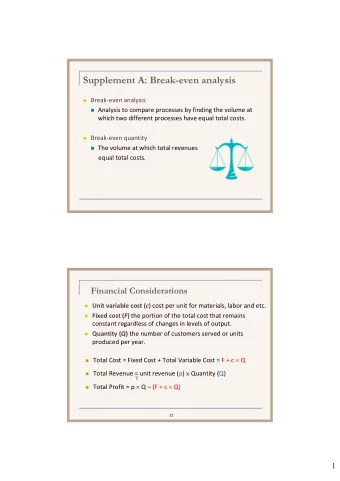
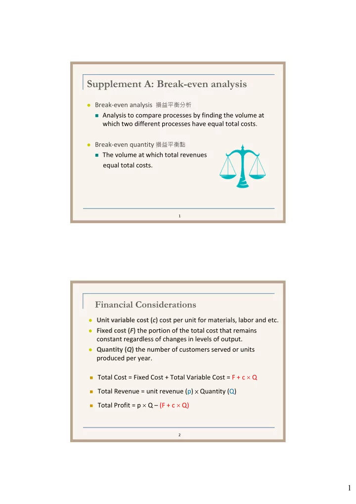
Supplement A: Break-even analysis  Break‐even analysis 損益平衡分析  Analysis to compare processes by finding the volume at which two different processes have equal total costs.  Break‐even quantity 損益平衡點  The volume at which total revenues equal total costs. 1 Financial Considerations  Unit variable cost ( c ) cost per unit for materials, labor and etc.  Fixed cost ( F ) the portion of the total cost that remains constant regardless of changes in levels of output.  Quantity ( Q ) t he number of customers served or units produced per year.  Total Cost = Fixed Cost + Total Variable Cost = F + c  Q  Total Revenue = unit revenue (p) × Quantity (Q)  Total Profit = p  Q – (F + c  Q) 2 1

Break-Even Analysis Total Profit = p × Q – (F + c × Q) Break‐even quantity F  Q = Total Revenue = Total Cost  p × Q = (F + c × Q)  p c F 3 Example A.1 A new procedure will be offered at $200 per patient. The fixed cost per year would be $100,000 with variable costs of $100 per patient. What is the break‐even quantity for this service? 400 – (2000, 400) F 100,000 Q = = Dollars (in thousands) Profit p – c 200 – 100 Total annual revenues 300 – (2000, 300) = 1,000 patients Total annual costs 200 – Break-even quantity 100 – Loss Fixed costs | | | | 500 1000 1500 2000 0 – Patients ( Q ) 4 2

Financial Analysis 水餃店原本雇用兼職人員包水餃，時薪 $150 。  現在考慮購買包水餃機以取代人工。  機器雙人操作，每小時可達600個水餃   Consider time value of money, present value=$150,000  Payback period=5 years  Annual interest rate=5%  Annual net cash flow= =PMT(5%,5,150000,0) =$34646 NPV 計算淨現值 5 Evaluating Alternatives: Make or Buy  F b : The fixed cost (per year) of the buy option  F m : The fixed cost of the make option c b : The variable cost (per unit) of the buy option  c m : The variable cost of the make option   Total cost to buy = F b + c b  Q  Total cost to make = F m + c m  Q  Q = F m – F b F b + c b  Q = F m + c m  Q c b – c m 6 3

Example A.3  A fast‐food restaurant is adding salads to the menu.  Make  Fixed costs: $12,000, variable costs: $1.50 per salad.  Buy  Preassembled salads could be purchased from a local supplier at $2.00 per salad. It would require additional refrigeration with an annual fixed cost of $2,400  The price to the customer will be the same.  Expected demand is 25,000 salads per year. Q = F m – F b = 12,000 – 2,400 = 19,200 salads < 25,000 c b – c m 2.0 – 1.5 7 Supplement B: Waiting Line Models Q: What are waiting lines and why do they form? A: Waiting Lines form due to a temporary imbalance between the demand for service and the capacity of the system to provide the service. 顧客異質性使供需短暫失調 Service system Customer Served population customers Waiting line Service facilities Priority rule 4

Structure of Waiting-Lines 1. An input, or customer population , that generates potential customers (single channel vs. multiple channels) 2. A waiting line of customers ( 號碼牌 ) 3. The service facility , consisting of a person (or crew), a machine (or group of machines), or both necessary to perform the service for the customer 4. A priority rule , which selects the next customer to be served by the service facility (FCFS) 5. Single phase vs. multiple phase 9 Random Arrivals (  T ) n e -  T Poisson arrival P n = for n = 0, 1, 2,… n ! distribution P n =Probability of n arrivals in T time periods  = Average numbers of arrivals per period 無尖離峰變化 e = 2.7183  = 2 arrivals per hour, T = 1 hour, and n = 4 arrivals. [2(1)] 4 e –2(1) 16 e –2 P 4 = = = 0.090 4! 24 10 5

Waiting Line Arrangements Single Line Service facilities Multiple Lines Service facilities Priority Rules  First‐come, first‐served (FCFS)  Earliest due date (EDD)  Shortest processing time (SPT)  Preemptive discipline (emergencies first) 12 6

Customer Service Times P ( t ≤ T ) = 1 – e –  T Exponential service time distribution μ = average number of customer completing service per period t = actual service time of the customer T = target service time  = 3 customers per hour, T = 10 minutes = 0.167 hour. P ( t ≤ 0.167 hour) = 1 – e –3(0.167) = 1 – 0.61 = 0.39 13 Waiting-Line Models to Analyze Operations  Balance costs (capacity, lost sales) against benefits (customer satisfaction) Satisfaction 1 0.8 sensitivity 0.6 0.4 0.2 0 t* perceived wait threshold 14 7

Single-Line Single-Server Model 單人服務  Single‐server, single waiting line, and only one phase  Assumptions are: 1. Customer population is infinite and patient 2. Customers arrive according to a Poisson distribution, with a mean arrival rate of  3. Service distribution is exponential with a mean service rate of  4. Mean service rate exceeds mean arrival rate  <  5. Customers are served FCFS 6. The length of the waiting line is unlimited 15 Single-Line Single-Server Model   = Average utilization of the system = < 1   n = Probability that n customers are in the system = (1–  )  n  L = Average number of customers in the system =  –  L q = Average number of customers in waiting = L –    L 1 W = Average time spent in the system, including service =  –  1 =  W W q = Average waiting time in line = W –  8

Little’s Law A fundamental law that relates the number of customers in a waiting‐line system to the arrival rate and average time in system  = arrival rate 流速 L customers average time W =  customer/hour in system Work‐in‐process L =  W 17 Single-Line Multiple-Server Model 平行服務 Service system has only one phase, multiple‐channels  Assumptions (in addition to single‐server model)  There are s identical servers  Exponential service distribution with mean 1/   s  should always exceed   18 9