Su Support'Vector'Machines Machine(Learning(Spring(2018 - PowerPoint PPT Presentation

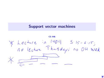
Su Support'Vector'Machines Machine(Learning(Spring(2018 March(5(2018 Kasthuri Kannan kasthuri.kannan@nyumc.org

Overview • Support Vector Machines for Classification – Linear Discrimination – Nonlinear Discrimination • SVM Mathematically • Extensions • Application in Drug Design • Data Classification • Kernel Functions 2

Definition One of the excellent classification system based on a mathematicaltechnique called convex optimization. ‘Support Vector Machine is a system for efficiently training linear learning machines in kernel-induced feature spaces, while respecting the insights of generalisation theory and exploiting optimisation theory.’ – AN INTRODUCTION TO SUPPORT VECTOR MACHINES (and other kernel-based learning methods) • N. Cristianini and J. Shawe-Taylor , Cambridge University Press 2000 ISBN: 0 521 78019 5 – Kernel Methods for Pattern Analysis • John Shawe-Taylor & Nello Cristianini Cambridge University Press, 2004 3

Dot product (aka inner product) a θ b a b a b cos ⋅ = θ Recall: If the vectors are orthogonal, dot product is zero. The scalar or dot product is, in some sense, a measure of similarity 4

Decision function for binary classification f ( x ) R ∈ f ( x ) 0 y 1 ≥ ⇒ = i i ( ) f x 0 y 1 < ⇒ = − i i 5

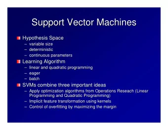
Support vector machines • SVMs pick best separating hyper plane according to some criterion – e.g. maximum margin • Training process is an optimisation • Training set is effectively reduced to a relatively small number of support vectors • Key words: optimization, kernels 6

Feature spaces • We may separate data by mapping to a higher- dimensional feature space – The feature space may even have an infinite number of dimensions! • We need not explicitly construct the new feature space – “Kernel trick” – Keeps the same computation time • Key observation that optimization involves dot products 7

Kernels • What are kernels? • We may use Kernel functions to implicitly map to a new feature space • Kernel functions: ( ) R K x 1 , x ∈ 2 • In SVMs kernels preserve the inner product in the new feature space. 8

Examples of kernels x ⋅ z Linear: Polynomial ( ) P x ⋅ z (non-linear) 2 / ( ) Gaussian 2 exp x − z − σ (non-linear) 9

Perceptron as linear separator • Binary classification can be viewed as the task of separating classes in feature space: w T x + b = 0 w T x + b > 0 f ( x ) = sign( w T x + b ) w T x + b < 0 10

Which of the linear separators is optimal? Tumor Normal 11

Best linear separator? Tumor Normal 12

Best linear separator? Tumor Normal 13

Best linear separator? Not so… Tumor Normal 14

Best linear separator? Possibly… Tumor Normal 15

Find closest points in convex hulls (3D)/convex polygon (2D) d c 16

Plane (3D)/line(2D) to bisect closest points w T x + b =0 w = d - c d c 17

Classification margin T + w x b • Distance from example data to the separator is r = w • Data closest to the hyper plane are support vectors . • Margin ρ of the separator is the width of separation between classes. ρ r 18

Maximum margin classification • Maximize the margin (good according to intuition and theory). • Implies that only support vectors are important; other training examples are ignorable. 19

Statistical learning theory • Misclassification error and the function complexity bound generalization error (prediction). • Maximizing margins minimizes complexity. • “Eliminates” overfitting. • Solution depends only on support vectors not number of attributes. 20

Margins and complexity Skinny margin is more flexible thus more complex. 21

Margins and complexity Fat margin is less complex. 22

Linear SVM • Assuming all data is at distance larger than 1 from the hyperplane, the following two constraints follow for a training set { ( x i , y i )} w T x i + b ≥ 1 if y i = 1 w T x i + b ≤ - 1 if y i = -1 • For support vectors, the inequality becomes an equality; then, since each example’s distance from the T + w x b 2 • hyperplane is the margin is: r ρ = = w w 23

Linear SVM We can formulate the problem: Find w and b such that 2 is maximized and for all { ( x i , y i )} ρ = w w T x i + b ≥ 1 if y i =1; w T x i + b ≤ - 1 if y i = -1 into quadratic optimization formulation: Find w and b such that Φ ( w ) = ½ w T w is minimized and for all { ( x i , y i )} y i ( w T x i + b ) ≥ 1 24

Solving the optimization problem Find w and b such that Φ ( w ) = ½ w T w is minimized and for all { ( x i , y i )} y i ( w T x i + b ) ≥ 1 • Need to optimize a quadratic function subject to linear constraints. • Quadratic optimization problems are a well-known class of mathematical programming problems, and many (rather intricate) algorithms exist for solving them. • The solution involves constructing a dual problem where a Lagrange multiplier α i is associated with every constraint in the primary problem: Find α 1 … α N such that Q ( α ) = Σ α i - ½ ΣΣ α i α j y i y j x iT x j is maximized and (1) Σ α i y i = 0 (2) α i ≥ 0 for all α i 25

The quadratic optimization problem solution • The solution has the form: w = Σ α i y i x i b = y k - w T x k for any x k such that α k ≠ 0 • Each non-zero α i indicates that corresponding x i is a support vector. • Then the classifying function will have the form: f ( x ) = Σ α i y i x iT x + b • Notice that it relies on an inner product between the test point x and the support vectors x i – we will return to this later! • Also keep in mind that solving the optimization problem involved computing the inner products x iT x j between all training points! 26

Soft margin classification • What if the training set is not linearly separable? • Slack variables ξ i can be added to allow misclassification of difficult or noisy examples. ξ i ξ i 27

Soft margin classification • The old formulation: Find w and b such that Φ ( w ) = ½ w T w is minimized and for all { ( x i , y i )} y i ( w T x i + b) ≥ 1 • The new formulation incorporating slack variables: Find w and b such that Φ ( w ) = ½ w T w + C Σ ξ i is minimized and for all { ( x i , y i )} y i ( w T x i + b ) ≥ 1- ξ i and ξ i ≥ 0 for all i • Parameter C can be viewed as a way to control overfitting. 28

Soft margin classification – solution • The dual problem for soft margin classification: Find α 1 … α N such that Q ( α ) = Σ α i - ½ ΣΣ α i α j y i y j x iT x j is maximized and (1) Σ α i y i = 0 (2) 0 ≤ α i ≤ C for all α i • Neither slack variables ξ i nor their Lagrange multipliers appear in the dual problem! • Again, x i with non-zero α i will be support vectors. But neither w nor b • Solution to the dual problem is: are needed explicitly for classification! w = Σ α i y i x i b= y k (1- ξ k ) - w T x k where k = argmax α k f ( x ) = Σ α i y i x iT x + b k 29

Theoretical justification for maximum margins • Vapnik has proved the following: The class of optimal linear separators has VC dimension h bounded from above as 2 D & # * ( h min , m 1 ≤ + % " ) ' 0 2 ρ ) ' $ ! where ρ is the margin, D is the diameter of the smallest sphere that can enclose all of the training examples, and m 0 is the dimensionality. • Intuitively, this implies that regardless of dimensionality m 0 we can minimize the VC dimension by maximizing the margin ρ . • Thus, complexity of the classifier is kept small regardless of dimensionality. 30

Linear SVM: Overview • The classifier is a separating hyperplane. • Most “important” training points are support vectors; they define the hyperplane. • Quadratic optimization algorithms can identify which training points x i are support vectors with non-zero Lagrangian multipliers α i . • Both in the dual formulation of the problem and in the solution training points appear only inside inner products: f ( x ) = Σ α i y i x iT x + b Find α 1 … α N such that Q ( α ) = Σ α i - ½ ΣΣ α i α j y i y j x iT x j is maximized and (1) Σ α i y i = 0 (2) 0 ≤ α i ≤ C for all α i 31

Non-linear SVMs • Datasets that are linearly separable with some noise work out great: x 0 • But what are we going to do if the dataset is just too hard? x 0 • How about… mapping data to a higher-dimensional space: x 2 x 0 32

Nonlinear classification ! # x = a , b " $ x i w = w 1 a + w 2 b ↓ ! # θ ( x ) = a , b , ab , a 2 , b 2 " $ θ ( x ) i w = w 1 a + w 2 b + w 3 ab + w 4 a 2 + w 5 b 2 33

Non-linear SVMs: Feature spaces • General idea: the original feature space can always be mapped to some higher-dimensional feature space where the training set is separable: Φ : x → φ ( x ) 34