String Search 5th September 2019 Petter Kristiansen Search - PowerPoint PPT Presentation
String Search 5th September 2019 Petter Kristiansen Search Problems have become increasingly important Vast ammounts of information The amount of stored digital information grows steadily (rapidly?) 3 zettabytes (10 21 = 1 000 000
String Search 5th September 2019 Petter Kristiansen
Search Problems have become increasingly important • Vast ammounts of information • The amount of stored digital information grows steadily (rapidly?) • 3 zettabytes (10 21 = 1 000 000 000 000 000 000 000 = trilliard) in 2012 • 4.4 zettabytes in 2013 • 44 zettabytes in 2020 (estimated) • 175 zettabytes in 2025 (estimated) • Search for a given pattern in DNA strings (about 3 giga-letters (10 9 ) in human DNA). • Google and similar search engines search for given strings (or sets of strings) on all registered web-pages. • Searching for similar patterns is also relevant e.g. for DNA-strings • The genetic sequences in organisms are changing over time because of mutations. • Searches for similar patterns are treated in Ch. 20.5. We will look at that in connection with Dynamic Programming
Definitions • An alphabet is a finite set of «symbols» A = { a 1 , a 2 , …, a k } . • A string S = S [0 : n- 1] or S = < s 0 s 1 … s n- 1 > of length n is a sequence of n symbols from A. String Search : Given two strings T (= Text) and P (= Pattern), P is usually much shorter than T. Decide whether P occurs as a (continuous) substring in T , and if so, find where it occurs. 0 1 2 … n -1 T [0: n -1] (Text) P [0: m -1] (Pattern)
Variants of String Search • Naive algorithm, no preprocessing of T or P • Assume that the length of T and P are n and m respectively • The naive algorithm is already a polynomial-time algorithm, with worst case execution time O ( n*m ) , which is also O ( n 2 ) . • Preprocessing of P (the pattern) for each new P • Prefix-search: The Knuth-Morris-Pratt algorithm • Suffix-search: The Boyer-Moore algorithm • Hash-based: The Karp-Rabin algorithm • Preprocess the text T (Used when we search the same text a lot of times (with different patterns), done to an extreme degree in search engines.) • Suffix trees: Data structure that relies on a structure called a Trie.
The naive algorithm (Prefix based) “Window” Searching forward n -1 0 1 2 … T [0: n -1] P [0: m -1]
The naive algorithm n -1 0 1 2 … T [0: n -1] P [0: m -1]
The naive algorithm n -1 0 1 2 … T [0: n -1] P [0: m -1]
The naive algorithm n-m n -1 0 1 2 … T [0: n -1] P [0: m -1]
The naive algorithm n-m n -1 0 1 2 … T [0: n -1] P [0: m -1] function NaiveStringMatcher ( P [0: m -1], T [0: n -1]) for s ← 0 to n - m do if T [ s : s + m - 1] = P then // is window = P? return ( s ) endif endfor return (-1) end NaiveStringMatcher
The naive algorithm n-m n -1 0 1 2 … T [0: n -1] P [0: m -1] function NaiveStringMatcher ( P [0: m -1], T [0: n -1]) } for s ← 0 to n - m do The for-loop is executed n – m + 1 times. if T [ s : s + m - 1] = P then // is window = P? Each string test has up to m symbol comparisons return ( s ) O ( nm ) execution time (worst case) endif endfor return (-1) end NaiveStringMatcher
The Knuth-Morris-Pratt algorithm (Prefix based) • There is room for improvement in the naive algorithm • The naive algorithm moves the window (pattern) only one character at a time. • But we can move it farther, based on what we know from earlier comparisons. Search forward 0 0 1 0 0 1 0 0 2 0 0 0 1 0 0 2 0 1 2 … 0 0 1 0 0 2 0 1
The Knuth-Morris-Pratt algorithm • There is room for improvement in the naive algorithm • The naive algorithm moves the window (pattern) only one character at a time. • But we can move it farther, based on what we know from earlier comparisons. Search forward 0 0 1 0 0 1 0 0 2 0 0 0 1 0 0 2 0 1 2 … 0 0 1 0 0 2 0 1
The Knuth-Morris-Pratt algorithm 0 0 1 0 0 1 0 0 2 0 0 0 1 0 0 2 0 1 2 … 0 0 1 0 0 2 0 1
The Knuth-Morris-Pratt algorithm 0 0 1 0 0 1 0 0 2 0 0 0 1 0 0 2 0 1 2 … 0 0 1 0 0 2 0 1 We move the pattern one step: Mismatch
The Knuth-Morris-Pratt algorithm 0 0 1 0 0 1 0 0 2 0 0 0 1 0 0 2 0 1 2 … 0 0 1 0 0 2 0 1 We move the pattern two steps: Mismatch
The Knuth-Morris-Pratt algorithm 0 0 1 0 0 1 0 0 2 0 0 0 1 0 0 2 0 1 2 … 0 0 1 0 0 2 0 1 3 We move the pattern three steps: Now, there is at least a match in the part of T where we had a match previously We can skip a number of tests and move the pattern more than one step before we start comparing characters again. • (3 in the above situation.) The key is that we know what the characters of T and P are up to the point where P and T got different. • ( T and P are equal up to this point.) For each possible index j in P, we assume that the first difference between P and T occurs at j , and from that compute • how far we can move P before the next string-comparison. It may well be that we never get an overlap like the one above, and we can then move P all the way to the point in T • where we found an inequality. This is the best case for the efficiency of the algorithm.
The Knuth-Morris-Pratt algorithm 0 1 i - d j i 0 0 1 0 0 1 0 0 2 0 0 0 1 0 0 2 0 1 2 … 0 1 j -1 j 0 0 1 0 0 2 0 1 0 0 1 0 0 2 0 1 0 j -2 j j - d j d j d j is the longest suffix of P [1 : j -1] that is also prefix of P [0 : j - 2] We know that if we move P less than j - d j steps, there can be no (full) match. And we know that, after this move, P [0: d j -1] will match the corresponding part of T . Thus we can start the comparison at d j in P and compare P [ d j : m -1] with the symbols from index i in T.
Idea behind the Knuth-Morris-Pratt algorithm • We will produce a table Next [0 : m- 1] that shows how far we can move P when we get a (first) mismatch at index j in P, j = 0,1,2, … , m -1 • But the array Next will not give this number directly. Instead, Next [ j ] will contain the new (and smaller value) that j should have when we resume the search after a mismatch at j in P (see below) • That is: Next [ j ] = j – <number of steps that P should be moved>, • or: Next [ j ] is the value that is named d j on the previous slide • After P is moved, we know that the first d j symbols of P are equal to the corresponding symbols in T (that’s how we chose d j ). • So, the search can continue from index i in T and Next [ j ] in P . • The array Next [] can be computed from P alone!
The Knuth-Morris-Pratt algorithm (5) 0 1 i - d j i 0 0 1 0 0 1 0 0 2 0 0 0 1 0 0 2 0 1 2 … (5) 0 1 j -1 j 0 0 1 0 0 2 0 1 0 0 1 0 0 2 0 1 0 j -2 j j - d j d j (2 = 5 - 3) we continue from here, this is Next[ 5 ]
function KMPStringMatcher ( P [0: m -1], T [0: n -1]) i ← 0 // indeks i T j ← 0 // indeks i P CreateNext ( P [0: m -1], Next [ n -1]) while i < n do if P [ j ] = T [ i ] then if j = m –1 then // check full match return ( i – m + 1) endif i ← i +1 j ← j +1 else j ← Next [ j ] if j = 0 then if T [ i ] ≠ P [0] then i ← i +1 endif endif endif endwhile return (-1) O ( n ) end KMPStringMatcher
Calculating the array Next[] from P function CreateNext ( P [0: m -1], Next [0: m -1]) … end CreateNext • This can be written straight-ahead with simple searches, and will then use time O ( m 2 ) . • A more clever approach finds the array Next in time O ( m ) . • We will look at the procedure in an exercise next week.
The Knuth-Morris-Pratt algorithm, example 0 0 1 0 0 1 0 0 2 0 0 0 1 0 0 2 0 1 2 … 0 0 1 0 0 2 0 1 The array Next for the string P above: j = 0 1 2 3 4 5 6 7 Next[ j ] = 0 0 1 1 1 2 0 1
The Knuth-Morris-Pratt algorithm, example 0 0 1 0 0 1 0 0 2 0 0 0 1 0 0 2 0 1 2 … 0 0 1 0 0 2 0 1 0 0 1 0 0 2 0 1 The array Next for the string P above: j = 0 1 2 3 4 5 6 7 Next[ j ] = 0 0 1 1 1 2 0 1
The Knuth-Morris-Pratt algorithm, example 0 0 1 0 0 1 0 0 2 0 0 0 1 0 0 2 0 1 2 … 0 0 1 0 0 2 0 1 0 0 1 0 0 2 0 1 0 0 1 0 0 2 0 1 The array Next for the string P above: j = 0 1 2 3 4 5 6 7 Next[ j ] = 0 0 1 1 1 2 0 1
The Knuth-Morris-Pratt algorithm, example 0 0 1 0 0 1 0 0 2 0 0 0 1 0 0 2 0 1 2 … 0 0 1 0 0 2 0 1 0 0 1 0 0 2 0 1 0 0 1 0 0 2 0 1 0 0 1 0 0 2 0 1 The array Next for the string P above: j = 0 1 2 3 4 5 6 7 Next[ j ] = 0 0 1 1 1 2 0 1
The Knuth-Morris-Pratt algorithm, example 0 0 1 0 0 1 0 0 2 0 0 0 1 0 0 2 0 1 2 … 0 0 1 0 0 2 0 1 0 0 1 0 0 2 0 1 0 0 1 0 0 2 0 1 0 0 1 0 0 2 0 1 The array Next for the string P above: j = 0 1 2 3 4 5 6 7 This is a linear algorithm: worst case runtime O ( n ). Next[ j ] = 0 0 1 1 1 2 0 1
The Boyer-Moore algorithm (Suffix based) • The naive algorithm, and Knuth-Morris-Pratt is prefix-based (from left to right through P ) • The Boyer-Moore algorithm (and variants of it) is suffix-based (from right to left in P ) • Horspool proposed a simplification of Boyer-Moore, and we will look at the resulting algorithm here. B M m a t c h e r _ s h i f t _ c h a r a c t e r _ e x … c h a r a c t e r
The Boyer-Moore algorithm (Horspool) Comparing from the end of P B M m a t c h e r _ s h i f t _ c h a r a c t e r _ e x … c h a r a c t e r
Recommend
More recommend
Explore More Topics
Stay informed with curated content and fresh updates.
