Stochastic models of protein production with feedback Renaud - PowerPoint PPT Presentation

Stochastic models of protein production with feedback Renaud Dessalles joint work with Vincent Fromion and Philippe Robert INRA Jouy-en-Josas - INRIA Rocquencourt (Fance) 16th. May 2016 1/29

Presentation Biological context Mathematical framework Equilibrium results Other aspects of the controlled model 2/29

Part 1 Biological context 3/29

Cells and proteins ▶ Cells: unit of life. ▶ Functional molecules: proteins ▶ Its goal: grow and divide. ▶ enzymes, wall, energy, etc. ▶ Produced from the genes 4/29

Protein production: A central mechanism Proteins represents: ▶ 50 % of the dry mass ▶ ∼ 3 million molecules ▶ ∼ 2000 different types ▶ from few dozens up to 10 5 proteins per type It needs to be duplicated in one cell cycle (approx. 30 min ) 5/29

Protein production: A central mechanism Proteins represents: ▶ 50 % of the dry mass ▶ ∼ 3 million molecules ▶ ∼ 2000 different types ▶ from few dozens up to 10 5 proteins per type It needs to be duplicated in one cell cycle (approx. 30 min ) 85% of the resources for protein production 5/29

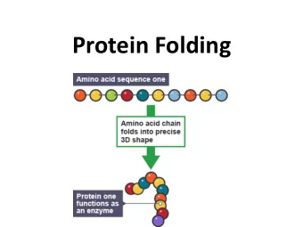
Classic protein production mechanism Protein production in 3 steps: 1. Gene regulation 2. Transcription: to produce mRNA 3. Translation: to produce proteins G e n e r e g u l a t i o n G O T r a n s c r i p t i o n A c t i v e g e n e T r a n s l a t i o n P r o t e i n mR N A I n a c t i v e g e n e D i l u t i o n 6/29

Highly variable process The protein production subject to high variability: ▶ Interior of bacteria: non-organized medium ▶ Mobility of compounds: through random diffusion ▶ Cellular mechanism: random collision between molecules 7/29

Highly variable process The protein production subject to high variability: ▶ Interior of bacteria: non-organized medium ▶ Mobility of compounds: through random diffusion ▶ Cellular mechanism: random collision between molecules Problem: 85% of the resources for the protein production, impacted by a large variability. 7/29

Highly variable process The protein production subject to high variability: ▶ Interior of bacteria: non-organized medium ▶ Mobility of compounds: through random diffusion ▶ Cellular mechanism: random collision between molecules Problem: 85% of the resources for the protein production, impacted by a large variability. A main issue for the bacteria: control the variability in protein production. 7/29

Protein production mechanism with feedback Production with feedback: the protein binds to its own gene. G e n e r e g u l a t i o n G O T r a n s c r i p t i o n A c t i v e g e n e T r a n s l a t i o n P r o t e i n mR N A I n a c t i v e g e n e D i l u t i o n More proteins ⇒ Gene more inactive A way to reduce variability? 8/29

Comparison of models Classical production vs Feedback production ▶ Conjecture: less variability in proteins with feedback production. 9/29

Comparison of models Classical production vs Feedback production ▶ Conjecture: less variability in proteins with feedback production. Our Goal Comparison of distributions of proteins in the two models. 9/29

Part 2 Mathematical framework 10/29

Markovian description Framework for protein production modeling: ▶ Rigney and Schieve (1977) ▶ Berg (1978) ▶ Paulsson (2005) Three types of events: ▶ Encounter between molecules ▶ Elongation of molecules ▶ Lifetime of molecules Assumption: Exponential times Each event occurs at exponential time. 11/29

The classical model G e n e r e g u l a t i o n G O A c t i v e g e n e I n a c t i v e g e n e I = 1 λ + λ − 1 1 I = 0 12/29

The classical model G e n e r e g u l a t i o n G O T r a n s c r i p t i o n A c t i v e g e n e mR N A I n a c t i v e g e n e λ 2 I I = 1 M λ + µ 2 M λ − 1 1 ∅ I = 0 12/29

The classical model G e n e r e g u l a t i o n G O T r a n s c r i p t i o n A c t i v e g e n e T r a n s l a t i o n P r o t e i n mR N A I n a c t i v e g e n e D i l u t i o n λ 2 I λ 3 M I = 1 M P λ + µ 2 M µ 3 P λ − 1 1 ∅ ∅ I = 0 12/29

Mean and variance for the classical model For the classical model, the mean and the variance are known Paulsson (2005) : ▶ Equality of flows gives λ + · λ 2 · λ 3 1 E [ P ] = λ + 1 + λ − µ 2 µ 3 1 ▶ Equilibrium equations give: ( λ 3 V ar [ P ] = E [ P ] 1 + µ 2 + µ 3 ) ( ( )) ( ) 1 − λ + λ + λ + 1 + λ − 1 + λ − + λ 2 λ 3 1 / 1 + µ 2 + µ 3 1 ( ) ( ) . λ + 1 + λ − λ + 1 + λ − ( µ 2 + µ 3 ) 1 + µ 2 1 + µ 3 13/29

The feedback model G e n e r e g u l a t i o n G O T r a n s c r i p t i o n A c t i v e g e n e T r a n s l a t i o n P r o t e i n mR N A I n a c t i v e g e n e D i l u t i o n λ 2 I F λ 3 M F I F = 1 M F P F � λ + µ 2 M F µ 3 P F λ − 1 P F 1 I F = 0 ∅ ∅ 14/29

Mean and variance for the Feedback model ▶ Equality of flows gives E [ P C ] = E [ I C ] · λ 2 · λ 3 . µ 2 µ 3 ▶ Problem : no known expression for E [ I C ] : ▶ the equality of flows on I C : � 1 E [ I C P C ] = λ + λ − 1 ( 1 − E [ I C ]) . Difficulties to make comparisons between the two models 15/29

Part 3 Equilibrium results 16/29

Scaling ▶ Introduction of a scaling: } Gene regulation timescale faster than the protein time scale Messenger RNA timescale 17/29

Scaling ▶ Introduction of a scaling: } Gene regulation timescale faster than the protein time scale Messenger RNA timescale Nλ 2 I N λ 3 M N F F I N M N P N F = 1 F F N � Nλ + Nµ 2 M N µ 3 P N 1 P N λ − 1 F F F I N F = 0 ∅ ∅ N scaling parameter 17/29

Effects of the scaling Example: Feedback model ▶ State of the model: ( ) I N F ( t ) , M N F ( t ) , P N F ( t ) ▶ I N F and M N F on a quick timescale. ▶ P N F on a slow timescale. I N F and M N F reach some equilibrium depending on the slow current P N F ( t ) state 18/29

Convergence of the gene regulation and the messengers τ N 1 : the first time of jump of P N F ; Starting at number of proteins x = P N F ( 0 ) ; 19/29

Convergence of the gene regulation and the messengers τ N 1 : the first time of jump of P N F ; Starting at number of proteins x = P N F ( 0 ) ; ▶ ( ) I N F ( t ) reaches its equilibrium quickly: [ ] N →∞ λ + I N F ( t ) | 0 < t < τ N 1 , P N 1 − − − − → E F ( 0 ) = x . 1 + � λ + λ − 1 x 19/29

Convergence of the gene regulation and the messengers τ N 1 : the first time of jump of P N F ; Starting at number of proteins x = P N F ( 0 ) ; ▶ ( ) I N F ( t ) reaches its equilibrium quickly: [ ] N →∞ λ + I N F ( t ) | 0 < t < τ N 1 , P N 1 − − − − → E F ( 0 ) = x . 1 + � λ + λ − 1 x ▶ ( ) M N F ( t ) reaches its equilibrium quickly: [ ] N →∞ λ + → λ 2 M N F ( t ) | 0 < t < τ N 1 , P N 1 F ( 0 ) = x − − − − · . E 1 + � µ 2 λ + λ − 1 x 19/29

Convergence of the gene regulation and the messengers τ N 1 : the first time of jump of P N F ; Starting at number of proteins x = P N F ( 0 ) ; ▶ ( ) I N F ( t ) reaches its equilibrium quickly: [ ] N →∞ λ + I N F ( t ) | 0 < t < τ N 1 , P N 1 − − − − → E F ( 0 ) = x . 1 + � λ + λ − 1 x ▶ ( ) M N F ( t ) reaches its equilibrium quickly: [ ] N →∞ λ + → λ 2 M N F ( t ) | 0 < t < τ N 1 , P N 1 F ( 0 ) = x − − − − · . E 1 + � µ 2 λ + λ − 1 x ▶ Rate of production of proteins tends to: λ + λ 3 · λ 2 1 · . µ 2 1 + � λ + λ − 1 x 19/29

Convergence of the models Theorem ( ) P N The process F ( t ) converges in distribution to a birth and death process with ( x number of proteins): λ + β x = λ 3 · λ 2 1 · and δ x = µ 3 x . µ 2 1 + � λ + λ − 1 x 20/29

Convergence of the models Theorem ( ) P N The process F ( t ) converges in distribution to a birth and death process with ( x number of proteins): λ + β x = λ 3 · λ 2 1 · and δ x = µ 3 x . µ 2 1 + � λ + λ − 1 x Idem for uncontrolled model: Theorem ( ) P N ( t ) The process converges in distribution to a birth and death process with ( x number of proteins): λ + β x = λ 3 · λ 2 1 · and δ x = µ 3 x . λ + µ 2 1 + λ − 1 20/29

Feature of the scaled models ▶ Equilibrium distributions. ▶ Classical model: P ∞ follow a Poisson distribution : ( λ 3 ) · λ 2 λ + P ∞ ∼ P 1 · µ 3 µ 2 λ + 1 + λ − 1 ▶ Feedback model: P ∞ follow the limit distribution ( λ 3 ) x x − 1 ∏ λ + 1 · λ 2 1 π F ( x ) = Z · x ! µ 3 µ 2 1 + � λ + λ − 1 i i = 0 21/29

Feature of the scaled models ▶ Equilibrium distributions. ▶ Classical model: P ∞ follow a Poisson distribution : ( λ 3 ) · λ 2 λ + P ∞ ∼ P 1 · µ 3 µ 2 λ + 1 + λ − 1 ▶ Feedback model: P ∞ follow the limit distribution ( λ 3 ) x x − 1 ∏ λ + 1 · λ 2 1 π F ( x ) = Z · x ! µ 3 µ 2 1 + � λ + λ − 1 i i = 0 Variance comparison V ar [ P ∞ ] = E [ P ∞ ] V ar [ P ∞ F ] ≤ E [ P ∞ and F ] 21/29