Stephen Taylor Vanderbilt University ICERM, Brown University, - PowerPoint PPT Presentation

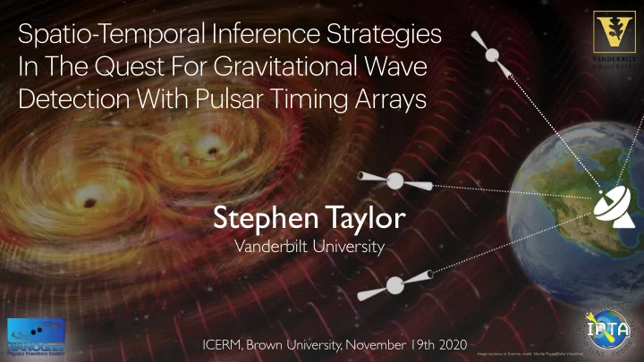
Spatio-Temporal Inference Strategies In The Quest For Gravitational Wave Detection With Pulsar Timing Arrays Stephen Taylor Vanderbilt University ICERM, Brown University, November 19th 2020 Image courtesy of Science , credit: Nicolle Rager Fuller [modified]

PTAs — The Elevator Pitch S. Taylor & C. Mingarelli, adapted from gwplotter.org (Moore, Cole, Berry 2014) and based on a figure in Mingarelli & Mingarelli (2018). Illustration of merging black holes adapted from R. Hurt/Caltech-JPL/EPA Stephen R. Taylor ICERM, Brown University, 11–19–2020

PTAs — The Elevator Pitch Cross-correlation signature of Gaussian stationary, isotropic, stochastic GW signal John Rowe Animation/Australia Telescope National Facility, CSIRO David Champion Stephen R. Taylor ICERM, Brown University, 11–19–2020

PTAs — The Elevator Pitch 1 1 f min = f max ∼ Big Bang = Supermassive Black Hole T obs 2 Δ t Galaxies grow via mergers over cosmic time ∼ 2 nHz ∼ 400 nHz Big Bang Supermassive black holes pair within galactic merger remnant. Stephen R. Taylor ICERM, Brown University, 11–19–2020

PTAs — The Elevator Pitch stochastic GW background coalescence timescale can be Myrs signal is present in entire data stream characteristic strain single resolvable binary binary merger 10 − 14 time “memory” offset time time oscillatory part 10 − 15 10 − 16 memory burst time 10 − 17 LISA band 10 − 8 10 − 7 10 − 6 10 − 9 frequency [Hz] Stephen R. Taylor ICERM, Brown University, 11–19–2020

Stephen R. Taylor ICERM, Brown University, 11–19–2020

From pulses to TOAs Verbiest & Shaifullah (2018) *TOA = times of arrival Stephen R. Taylor ICERM, Brown University, 11–19–2020

good timing solution error in position Creating a timing error in frequency derivative unmodeled proper motion ephemeris Lorimer & Kramer (2005) Stephen R. Taylor ICERM, Brown University, 11–19–2020

⃗ ⃗ ⃗ ⃗ ⃗ Pulsar-timing Data Model random Gaussian processes t det + ⃗ t TOA = t stoch t TOA − ⃗ δ t ≡ t det ( β 0 ) Timing residuals Deterministic Stochastic timing ephemeris per-pulsar achromatic red noise per-pulsar white noise transient noise features per-pulsar chromatic red noise single resolvable GW signals GWB interpulsar-correlated achromatic processes Stephen R. Taylor ICERM, Brown University, 11–19–2020

Sources of noise Verbiest & Shaifullah (2018) Stephen R. Taylor ICERM, Brown University, 11–19–2020

Sources of noise Verbiest & Shaifullah (2018) Stephen R. Taylor ICERM, Brown University, 11–19–2020

Sources of noise Verbiest & Shaifullah (2018) Stephen R. Taylor ICERM, Brown University, 11–19–2020

Pulsar-timing Data Model δ t = δ t tm + δ t white + δ t red • Intrinsic low-frequency processes • Rotational instabilities lead to random • Deviations around best- f it of timing walk in phase, period, period-derivative ephemeris • Radio-frequency dependent dispersion- measure variations • White noise • TOA measurement uncertainties • Spatially-correlated low-frequency • Extra unaccounted white-noise from processes receivers • Stochastic variations in time standards • Pulse phase “jitter” • Solar-system ephemeris errors • Gravitational-wave background Stephen R. Taylor ICERM, Brown University, 11–19–2020

⃗ ⃗ ⃗ ⃗ ⃗ ⃗ ⃗ ⃗ Timing Ephemeris ∂ t det, i ∑ × ( β j − β 0, j ) t det, i ( β ) = t det, i ( β 0 ) + ∂ β j j β 0 t det ( β ) = t det ( β 0 ) + M ϵ Timing ephemeris design matrix for linear o ff sets Stephen R. Taylor ICERM, Brown University, 11–19–2020

Timing Ephemeris Temporal behavior of timing ephemeris basis Stephen R. Taylor ICERM, Brown University, 11–19–2020

White Noise (1/2) • Flat power-spectral density across all sampling frequencies • No inter-pulsar correlations ⟨ n i , μ n j , ν ⟩ = F 2 μ σ 2 i δ ij δ μν + Q 2 μ δ ij δ μν EFAC = Extra FACtor to correct uncertainties EQUAD = Extra QUADrature “Radiometer noise”— pulse template f itting uncertainties Stephen R. Taylor ICERM, Brown University, 11–19–2020

White Noise (2/2) • Fitting a template to a f inite-pulse folded Radiometer, EFAC, EQUAD observation can give “jitter” errors ECORR • Simultaneous observations across many radio sub-bands in an epoch will have epoch correlated jitter errors j , ν ⟩ = J 2 ⟨ n J i , μ n J μ δ e ( i ) e ( j ) δ μν ECORR = Extra CORRelated white noise Stephen R. Taylor ICERM, Brown University, 11–19–2020

Red Processes (1/5) Stephen R. Taylor ICERM, Brown University, 11–19–2020

⃗ ⃗ ⃗ ⃗ ⃗ ⃗ Red Processes (2/5) ⟨ δ t i δ t j ⟩ = C ( | t i − t j | ) • Time-domain covariance matrix is large and dense • But we only care abut the lowest frequencies δ t red = F a • Use a rank-reduced formalism for covariance T a T ⟩ F T ⟨ red ⟩ = F ⟨ δ t red δ t a C = F ϕ F T Stephen R. Taylor ICERM, Brown University, 11–19–2020

⃗ ⃗ Red Processes (3/5) δ t red = F a Fourier design matrix over small number of modes Stephen R. Taylor ICERM, Brown University, 11–19–2020

⃗ ⃗ ⃗ ⃗ ⃗ ⃗ ⃗ ⃗ Red Processes (4/5) δ t red = F a Fourier coe fg icients exp ( − 1 a ) η ) − 1 a T ϕ ( 2 p ( η ) = a | det(2 πϕ ( η )) [ ϕ ] ( ak )( bj ) = Γ ab ρ k δ kj + κ ak δ kj δ ab Intrinsic red-noise PSD GWB PSD Overlap Reduction Function Stephen R. Taylor ICERM, Brown University, 11–19–2020

Red Processes (5/5) • power laws • per frequency ρ ( f ) = S ( f ) Δ f = h c ( f ) 2 • GP emulators 1 GWB PSD 12 π 2 f 3 T Γ ab ∝ (1 + δ ab ) ∫ S 2 Ω ) [ F + Ω ) ] d 2 ̂ Ω P ( ̂ a ( ̂ b ( ̂ a ( ̂ b ( ̂ GWB ORF Ω ) + F × Ω ) F × Ω ) F + PTA overlap reduction function for Gaussian stationary, isotropic stochastic GWB “Hellings & Downs Curve” (1983) Stephen R. Taylor ICERM, Brown University, 11–19–2020

⃗ ⃗ ⃗ ⃗ ⃗ ⃗ The PTA Likelihood a + U ⃗ δ t = M ϵ + F j + n white noise small linear perturbations jitter low-frequency processes around best-fit timing solution in Fourier basis [ M ] = N TOA × N tm [ F ] = N TOA × 2 N freqs [ U ] = N TOA × N epochs [ ⃗ [ a ] = 2 N freqs j ] = N epochs [ ϵ ] = N tm “U” has block diagonal structure, “M” is matrix of TOA derivatives “F” has columns of sines and wrt timing-model parameters with ones filling each block cosines for each frequency ~ few tens ~ couple of hundred ~ few tens Lentati et al. (inc Taylor) (2013) van Haasteren & Vallisneri (2014a,b) Stephen R. Taylor ICERM, Brown University, 11–19–2020

⃗ ⃗ ⃗ ⃗ ⃗ ⃗ ⃗ ⃗ ⃗ ⃗ ⃗ ⃗ ⃗ ⃗ ⃗ ⃗ ⃗ ⃗ ⃗ ⃗ ⃗ The PTA Likelihood exp ( − 1 n ) n T N − 1 2 Start with Gaussian white noise likelihood p ( n ) = det(2 π N ) exp [ − 1 N − 1 ( j ) ] T 2 ( j ) a − U ⃗ a − U ⃗ δ t − M ϵ − F δ t − M ϵ − F a , ⃗ p ( ϵ , j ) = δ t | det(2 π N ) exp [ − 1 N − 1 ( a + U ⃗ b = M ϵ + F T j b ) b ) ] T 2 ( δ t − T δ t − T   ✏ p ( b ) = T = [ M U ] δ t | F a b =   det(2 π N ) j Stephen R. Taylor ICERM, Brown University, 11–19–2020

⃗ ⃗ ⃗ ⃗ ⃗ ⃗ ⃗ ⃗ ⃗ ⃗ ⃗ ⃗ ⃗ ⃗ ⃗ ⃗ ⃗ ⃗ ⃗ ⃗ ⃗ ⃗ The PTA Likelihood But we’re describing all stochastic terms as random Gaussian processes… exp ( − 1 b ) b T B − 1 2 p ( b | η ) = det(2 π B ) hierarchical modelling δ t ) ∝ p ( p ( η , b | δ t | b ) p ( b | η ) p ( η ) δ t ) = ∫ p ( (analytically!) marginalize over coefficients p ( η | η | δ t ) d b exp ( − 1 δ t ) T C − 1 δ t 2 C = N + TBT T δ t ) ∝ p ( η | p ( η ) det(2 π C ) Stephen R. Taylor ICERM, Brown University, 11–19–2020

The PTA Likelihood C = N + TBT T what are we actually doing here? N f ∑ [ TBT T ] ( ab ), τ = this is just the Wiener-Khinchin theorem! [ ϕ ] ab cos(2 π k τ / T ) k Woodbury lemma C − 1 = ( N − 1 + TBT T ) − 1 = N − 1 − N − 1 T ( B − 1 + T T N − 1 T ) − 1 T T N − 1 Much easier and faster than inversion N TOA × N TOA Stephen R. Taylor ICERM, Brown University, 11–19–2020

The PTA Likelihood A GW , γ GW ρ GW ρ RN ρ DM A RN , γ RN A DM , γ DM c lm σ WN P (ˆ a RN a DM Ω ) GW EQUAD β a GW EFAC ECORR t RN t DM t GW t WN t TM courtesy J. Ellis t TOA pulsars Without inter-pulsar correlations The PTA Bayesian Network [~ tens of ms] With inter-pulsar correlations [~few seconds] Stephen R. Taylor ICERM, Brown University, 11–19–2020

NANOGrav 12.5yr Dataset Search (arXiv:2009.04496), corresponding author: Joe Simon (JPL / CU-Boulder) Stephen R. Taylor ICERM, Brown University, 11–19–2020

NANOGrav 12.5yr Dataset Search A Common-spectrum Process (arXiv:2009.04496), corresponding author: Joe Simon (JPL / CU-Boulder) A steep-spectrum process in common across NANOGrav’s 45-pulsar array with max baseline of 12.9 years Stephen R. Taylor ICERM, Brown University, 11–19–2020