Stein Variational Newton & other Sampling-Based Inference - PowerPoint PPT Presentation
Stein Variational Newton & other Sampling-Based Inference Methods Robert Scheichl Interdisciplinary Center for Scientific Computing & Institute of Applied Mathematics Universit at Heidelberg Collaborators: G. Detommaso (Bath); T.
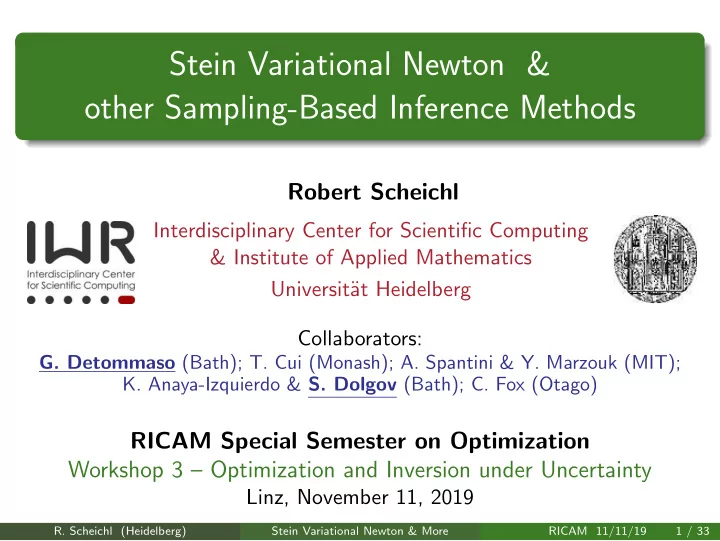
Stein Variational Newton & other Sampling-Based Inference Methods Robert Scheichl Interdisciplinary Center for Scientific Computing & Institute of Applied Mathematics Universit¨ at Heidelberg Collaborators: G. Detommaso (Bath); T. Cui (Monash); A. Spantini & Y. Marzouk (MIT); K. Anaya-Izquierdo & S. Dolgov (Bath); C. Fox (Otago) RICAM Special Semester on Optimization Workshop 3 – Optimization and Inversion under Uncertainty Linz, November 11, 2019 R. Scheichl (Heidelberg) Stein Variational Newton & More RICAM 11/11/19 1 / 33
Inverse Problems Data Parameter y = F ( x ) + e forward model (PDE) observation/model errors R. Scheichl (Heidelberg) Stein Variational Newton & More RICAM 11/11/19 2 / 33
Inverse Problems Data Parameter y = F ( x ) + e forward model (PDE) observation/model errors y ∈ R N y Data y are limited in number, noisy, and indirect. x ∈ X Parameter x often a function (discretisation needed). F : X → R N y Continuous, bounded, and sufficiently smooth. R. Scheichl (Heidelberg) Stein Variational Newton & More RICAM 11/11/19 2 / 33
Bayesian interpretation The (physical) model gives π ( y | x ), the conditional probability of observing y given x . However, to predict, control, optimise or quantify uncertainty, the interest is often really in π ( x | y ), the conditional probability of possible causes x given the observed data y – the inverse problem : R. Scheichl (Heidelberg) Stein Variational Newton & More RICAM 11/11/19 3 / 33
Bayesian interpretation The (physical) model gives π ( y | x ), the conditional probability of observing y given x . However, to predict, control, optimise or quantify uncertainty, the interest is often really in π ( x | y ), the conditional probability of possible causes x given the observed data y – the inverse problem : π pos ( x ) := π ( x | y ) ∝ π ( y | x ) π pr ( x ) � �� � Bayes’ rule R. Scheichl (Heidelberg) Stein Variational Newton & More RICAM 11/11/19 3 / 33
Bayesian interpretation The (physical) model gives π ( y | x ), the conditional probability of observing y given x . However, to predict, control, optimise or quantify uncertainty, the interest is often really in π ( x | y ), the conditional probability of possible causes x given the observed data y – the inverse problem : π pos ( x ) := π ( x | y ) ∝ π ( y | x ) π pr ( x ) � �� � Bayes’ rule Extract information from π pos (means, covariances, event probabilities, predictions) by evaluating posterior expectations: � E π pos [ h ( x )] = h ( x ) π pos ( x ) dx R. Scheichl (Heidelberg) Stein Variational Newton & More RICAM 11/11/19 3 / 33
Bayes’ Rule and Classical Inversion Classically [Hadamard, 1923]: Inverse map “ F − 1 ” ( y → x ) is typically ill-posed, i.e. lack of (a) existence , (b) uniqueness or (c) boundedness R. Scheichl (Heidelberg) Stein Variational Newton & More RICAM 11/11/19 4 / 33
Bayes’ Rule and Classical Inversion Classically [Hadamard, 1923]: Inverse map “ F − 1 ” ( y → x ) is typically ill-posed, i.e. lack of (a) existence , (b) uniqueness or (c) boundedness least squares solution ˆ x is maximum likelihood estimate prior distribution π pr “acts” as regulariser – well-posedness ! solution of regularised least squares problem is maximum a posteriori (MAP) estimator R. Scheichl (Heidelberg) Stein Variational Newton & More RICAM 11/11/19 4 / 33
Bayes’ Rule and Classical Inversion Classically [Hadamard, 1923]: Inverse map “ F − 1 ” ( y → x ) is typically ill-posed, i.e. lack of (a) existence , (b) uniqueness or (c) boundedness least squares solution ˆ x is maximum likelihood estimate prior distribution π pr “acts” as regulariser – well-posedness ! solution of regularised least squares problem is maximum a posteriori (MAP) estimator However, in the Bayesian setting, the full posterior π pos contains more information than the MAP estimator alone, e.g. the posterior covariance matrix reveals components of x that are (relatively) more or less certain. R. Scheichl (Heidelberg) Stein Variational Newton & More RICAM 11/11/19 4 / 33
Bayes’ Rule and Classical Inversion Classically [Hadamard, 1923]: Inverse map “ F − 1 ” ( y → x ) is typically ill-posed, i.e. lack of (a) existence , (b) uniqueness or (c) boundedness least squares solution ˆ x is maximum likelihood estimate prior distribution π pr “acts” as regulariser – well-posedness ! solution of regularised least squares problem is maximum a posteriori (MAP) estimator However, in the Bayesian setting, the full posterior π pos contains more information than the MAP estimator alone, e.g. the posterior covariance matrix reveals components of x that are (relatively) more or less certain. Possible to sample/explore via Metropolis-Hastings MCMC (in theory) R. Scheichl (Heidelberg) Stein Variational Newton & More RICAM 11/11/19 4 / 33
Variational Bayes (as opposed to Metropolis-Hastings MCMC) Aim to characterise the posterior distribution (density π pos ) analytically (at least approximately) for more efficient inference. R. Scheichl (Heidelberg) Stein Variational Newton & More RICAM 11/11/19 5 / 33
Variational Bayes (as opposed to Metropolis-Hastings MCMC) Aim to characterise the posterior distribution (density π pos ) analytically (at least approximately) for more efficient inference. This is a challenging task since: x ∈ R d is typically high-dimensional (e.g., discretised function) π pos is in general non-Gaussian (even if π pr and observation noise are Gaussian) evaluations of likelihood may be expensive (e.g., solution of a PDE) R. Scheichl (Heidelberg) Stein Variational Newton & More RICAM 11/11/19 5 / 33
Variational Bayes (as opposed to Metropolis-Hastings MCMC) Aim to characterise the posterior distribution (density π pos ) analytically (at least approximately) for more efficient inference. This is a challenging task since: x ∈ R d is typically high-dimensional (e.g., discretised function) π pos is in general non-Gaussian (even if π pr and observation noise are Gaussian) evaluations of likelihood may be expensive (e.g., solution of a PDE) Key Tools Transport Maps, Optimisation , Principle Component Analysis, Model Order Reduction, Hierarchies, Sparsity, Low Rank Approximation R. Scheichl (Heidelberg) Stein Variational Newton & More RICAM 11/11/19 5 / 33
Deterministic Couplings of Probability Measures T η π R. Scheichl (Heidelberg) Stein Variational Newton & More RICAM 11/11/19 6 / 33
Deterministic Couplings of Probability Measures T η π Core idea [Moselhy, Marzouk, 2012] Choose a reference distribution η (e.g., standard Gaussian) Seek transport map T : R d → R d such that T ♯ η = π (or equivalently its inverse S = T − 1 ) R. Scheichl (Heidelberg) Stein Variational Newton & More RICAM 11/11/19 6 / 33
Deterministic Couplings of Probability Measures T η π Core idea [Moselhy, Marzouk, 2012] Choose a reference distribution η (e.g., standard Gaussian) Seek transport map T : R d → R d such that T ♯ η = π (or equivalently its inverse S = T − 1 ) In principle, enables exact (independent, unweighted) sampling! R. Scheichl (Heidelberg) Stein Variational Newton & More RICAM 11/11/19 6 / 33
Deterministic Couplings of Probability Measures T η π Core idea [Moselhy, Marzouk, 2012] Choose a reference distribution η (e.g., standard Gaussian) Seek transport map T : R d → R d such that T ♯ η = π (or equivalently its inverse S = T − 1 ) In principle, enables exact (independent, unweighted) sampling! Satisfying these conditions only approximately can still be useful! R. Scheichl (Heidelberg) Stein Variational Newton & More RICAM 11/11/19 6 / 33
Variational Inference Goal: Sampling from target density π ( x ) R. Scheichl (Heidelberg) Stein Variational Newton & More RICAM 11/11/19 7 / 33
Variational Inference Goal: Sampling from target density π ( x ) Given a reference density p , find an invertible map ˆ T such that ˆ D KL ( p � T − 1 T := argmin D KL ( T ♯ p � π ) = argmin π ) ♯ T T where � � � � T − 1 ( x ) ∇ x T − 1 ( x ) T ♯ ( x ):= p | det | . . . push-forward of p � � p ( x ) � D KL ( p � q ):= log p ( x ) d x . . . Kullback-Leibler divergence q ( x ) R. Scheichl (Heidelberg) Stein Variational Newton & More RICAM 11/11/19 7 / 33
Variational Inference Goal: Sampling from target density π ( x ) Given a reference density p , find an invertible map ˆ T such that ˆ D KL ( p � T − 1 T := argmin D KL ( T ♯ p � π ) = argmin π ) ♯ T T where � � � � T − 1 ( x ) ∇ x T − 1 ( x ) T ♯ ( x ):= p | det | . . . push-forward of p � � p ( x ) � D KL ( p � q ):= log p ( x ) d x . . . Kullback-Leibler divergence q ( x ) Advantage of using D KL : do not need normalising constant for π R. Scheichl (Heidelberg) Stein Variational Newton & More RICAM 11/11/19 7 / 33
Recommend
More recommend
Explore More Topics
Stay informed with curated content and fresh updates.
