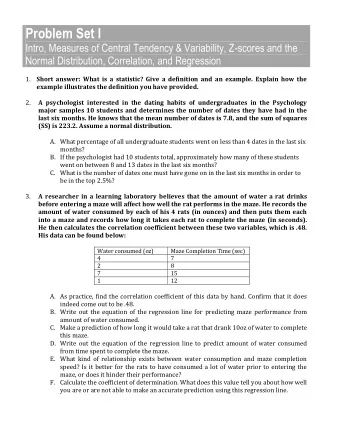
Statistics, Measures of Central Tendency I We are considering a - PowerPoint PPT Presentation

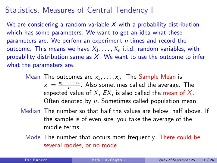
Statistics, Measures of Central Tendency I We are considering a random variable X with a probability distribution which has some parameters. We want to get an idea what these parameters are. We perfom an experiment n times and record the outcome. This means we have X 1 , . . . , X n i.i.d. random variables, with probability distribution same as X . We want to use the outcome to infer what the parameters are. Mean The outcomes are x 1 , . . . , x n . The Sample Mean is x := x 1 + ··· + x n . Also sometimes called the average. The n expected value of X , EX , is also called the mean of X . Often denoted by µ. Sometimes called population mean. Median The number so that half the values are below, half above. If the sample is of even size, you take the average of the middle terms. Mode The number that occurs most frequently. There could be several modes, or no mode. Dan Barbasch Math 1105 Chapter 9 Week of September 25 1 / 24

Statistics, Measures of Central Tendency II Example You have a coin for which you know that P ( H ) = p and P ( T ) = 1 − p . You would like to estimate p . You toss it n times. You count the number of heads. The sample mean should be an estimate of p . EX = p , and E ( X 1 + · · · + X n ) = np . So � X 1 + · · · + X n � E = p . n Dan Barbasch Math 1105 Chapter 9 Week of September 25 2 / 24

Descriptive Statistics I Frequency Distribution Divide into a number of equal disjoint intervals. For each interval count the number of elements in the sample occuring. Histogram see the next slide Grouped Data Mean Essentially calculate the mean of the frequency distribution. Intervals are used, rather than single values. It is assumed that all these values are located at the midpoint of the interval. The letter x M is used to represent the midpoints and f represents the frequencies: � f i x M , i n Frequency Polygon Connect the middles of the tops of each interval. Dan Barbasch Math 1105 Chapter 9 Week of September 25 3 / 24

Histogram A histogram is a graphical representation of the distribution of numerical data. It is a kind of bar graph. To construct a histogram, the first step is to ”bin” the range of values, that is, divide the entire range of values into a series of intervals, and then count how many values fall into each interval. The bins are usually specified as consecutive, non-overlapping intervals of a variable. The bins (intervals) must be adjacent, and are often (but are not required to be) of equal size. Bin Count − 3 . 5 − 2 . 51 9 − 2 . 5 − 1 . 51 32 − 1 . 5 − 0 . 51 109 − 0 . 5 − 0 . 49 180 0 . 5 − 1 . 49 132 1 . 5 − 2 . 49 34 2 . 5 − 3 . 49 4 ( − 3) · 9+( − 2) · 32+( − 1) · 109+ · (0)180+1 · 132+2 · 34+3 · 4 Mean: 500 Dan Barbasch Math 1105 Chapter 9 Week of September 25 4 / 24

Example The table on the next page gives the number of days in June and July of recent years in which the temperature reached 90 degrees or higher in New Yorks Central Park. Source: The New York Times and Accuweather.com. a. Prepare a frequency distribution with a column for intervals and frequencies. Use seven intervals, starting with [0 4]. b. Sketch a histogram and a frequency polygon, using the intervals in part a. c. Find the mean for the original data. d. Find the mean using the grouped data from part a. e. Explain why your answers to parts c and d are different. f. Find the median and the mode for the original data. Dan Barbasch Math 1105 Chapter 9 Week of September 25 5 / 24

fi Temperature Data Year Days Year Days Year Days 1972 11 1985 4 1998 5 1973 8 1986 8 1999 24 1974 11 1987 14 2000 3 1975 3 1988 21 2001 4 1976 8 1989 10 2002 13 1977 11 1990 6 2003 11 1978 5 1991 21 2004 1 1979 7 1992 4 2005 12 1980 12 1993 25 2006 5 1981 12 1994 16 2007 4 1982 11 1995 14 2008 10 1983 20 1996 0 2009 0 1984 7 1997 10 2010 20 Dan Barbasch Math 1105 Chapter 9 Week of September 25 6 / 24

Measures of Variation Summary of Section 9.2 Range The difference Largest Data - Smallest Data in a Sample. Deviation from the Mean � x 2 i − nx 2 � ( x i − x ) 2 1 Variance σ 2 = s 2 = = n − 1 √ n − 1 2 Standard Deviation σ = s = s 2 These are random variables called Sample Variance and Sample Standard Deviation. For a random variable X , µ = E ( X ) is called the mean. The variance Var ( X ) is σ 2 = Var ( X ) = E (( X − µ ) 2 ). Main Property/ Explanation for dividing by n − 1: If X i are i.i.d with distribution X , then if you set S 2 = � ( X i − X ) 2 , its n − 1 expected value is E ( S 2 ) = σ 2 . This is not true for the standard deviation, E ( S ) � = σ. �� f i x 2 M , i − nx 2 Grouped Data s = . n − 1 Dan Barbasch Math 1105 Chapter 9 Week of September 25 7 / 24

Examples I Example (Range) Data 15 , − 3 , 4 , 7 , 18. The smallest is − 3, the largest 18 so Range = 18 − ( − 3) = 21 . Always a nonnegative number. Example (Deviation from the Mean) In the previous example, x = 15 − 3+4+7+18 = 8 . 2. So 5 15 − 8 . 2 = 6 . 8 , − 3 − 8 . 2 = − 11 . 2 , 4 − 8 . 2 = − 3 . 8 , 7 − 8 . 2 = − 1 . 2 , 18 − 8 . 2 = 9 . 8 . Example (Variance and Standard Deviation) s 2 = 6 . 8 2 +11 . 2 2 +3 . 8 2 +1 . 2 2 +9 . 8 2 = 15 2 +3 2 +4 2 +7 2 +18 2 − 5 · 8 . 2 2 √ 4 4 s 2 . s = Dan Barbasch Math 1105 Chapter 9 Week of September 25 8 / 24

Examples II Example (Binomial Distribution) P ( X = 1) = p , P ( X = 0) = 1 − p . Then µ = E ( X ) = p , and σ 2 = E (( X − p ) 2 ) = (1 − p ) 2 p + (0 − p ) 2 (1 − p ) = p (1 − p ) . This is the same as E ( X 2 − p 2 ) = (1 − p 2 ) p + ( − p 2 )(1 − p ) = (1 − p ) p . Remark: Note that the formula for variance and standard deviation only holds for n > 2 . Otherwise, for n = 1 , you would be dividing by 0. For one random variable, the variance is defined as Var ( X ) = E (( X − E ( X )) 2 ) . For X 1 , X 2 , , two independent random variables, Var ( X 1 + X 2 ) = Var ( X 1 ) + Var ( X 2 ) . Suppose X is a random variable. We can write a table . . . X a 1 a 2 a n P ( X ) p 1 p 2 . . . p n Dan Barbasch Math 1105 Chapter 9 Week of September 25 9 / 24

Examples III For the expected value µ = E ( X ) , you multiply the two terms in each column, and add � a i × p n = a 1 p 1 + · · · + a n p n . i In a spreadsheet program, the data would be in columns and you would add over the products from the rows. You use a command like sumproduct to perform the operation. If you have some other variable like ( X − µ ) 2 , you would use the values ( a i − µ ) 2 and the same p i . Dan Barbasch Math 1105 Chapter 9 Week of September 25 10 / 24

Examples IV Example 2 3 − 1 1 X X 2 4 9 1 1 ( X − µ ) 2 (2 − 1 / 4) 2 (3 − 1 / 4) 2 ( − 1 − 1 / 4) 2 (1 − 1 / 4) 2 P ( X ) 1 / 2 1 / 8 1 / 4 1 / 8 Computing the expected values is below. µ = E ( X ) = (2) × (1 / 2) + (3) × (1 / 8) + ( − 1) × (1 / 4) + (1) × (1 / 8) = 1 / 4 . Var ( X ) =(2 − 1 / 4) 2 · (1 / 2) + (3 − 1 / 4) 2 · (1 / 8) + ( − 1 − 1 / 4) 2 · (1 / 4)+ +(1 − 1 / 4) 2 · (1 / 8) = 47 / 16 . Dan Barbasch Math 1105 Chapter 9 Week of September 25 11 / 24

Grouped Data Example (Grouped Data) Interval Frequency Midpoint x M 30-39 1 34.5 40-49 6 44.5 50-59 13 54.5 60-69 22 64.5 70-79 17 74.5 80-89 13 84.5 90-99 8 94.5 Find the standard deviation of these grouped data. In this case you must sum the x 2 M multiplied by the frequencies, and subtract 80 × x where x is for the full sample, (which is not in the table, you must get it from the full data). Dan Barbasch Math 1105 Chapter 9 Week of September 25 12 / 24

Chebyshev’s and Markov’s Inequality I P ( X ≥ a ) ≤ E ( X ) Markov . a P ( | X − µ | ≥ k σ ) ≤ 1 Chebyshev . k 2 In words, the probability that X is more than k standard deviations away from the mean is less than 1 / k 2 . Dan Barbasch Math 1105 Chapter 9 Week of September 25 13 / 24

Chebyshev’s and Markov’s Inequality II Example (from the practice prelim) 8. (14 points) Assume that the height in inches of American women follows a normal distribution with mean Mu = 64 ′′ (5’4”) and standard deviation σ = 3 ′′ . (a) (3 points) How many standard deviations above or below the mean is a height of 72” (6’0”)? (b) (4 points) What fraction of women are taller than 6 feet? (c) (4 points) In a room with 30 women, what is the probability that at least one of them is taller than 6 feet? (d) (3 points) What assumptions did you make when answering part (c)? Are there circumstances under which those assumptions would not be justified? Dan Barbasch Math 1105 Chapter 9 Week of September 25 14 / 24

Chebyshev’s and Markov’s Inequality III Answer. Say we don’t know what distribution it is. We can still use Markov’s and Chebyshev’s inequality. (a) 72 − 64 = 8 3 , so closer to 3. Use 73 to get 3. 3 (b) Markov’s inequality says P ( X ≥ 73) ≤ 64 73 . To use Chebyshev’s inequality we must write | X − 64 | ≥ 3 σ . Then P ( | X − 64 | ≥ 3 σ ) ≤ 1 9 . In other words, k = 3. This includes not just X ≥ 73 , but also X ≤ 55 . Still we can say the probability is less than 1 / 9 , because | X − 64 | ≥ 9 is larger than X − 64 ≥ 9. (c) 1 − P ( none are taller than 6 ) = 1 − (1 − P ( one is not taller than 6 )) 30 . Dan Barbasch Math 1105 Chapter 9 Week of September 25 15 / 24