Statistics and Data Analysis Descriptive Statistics (2): - PowerPoint PPT Presentation
Central tendency Variability Correlation Statistics and Data Analysis Descriptive Statistics (2): Summarization Ling-Chieh Kung Department of Information Management National Taiwan University Descriptive Statistics 1 / 33 Ling-Chieh Kung
Central tendency Variability Correlation Statistics and Data Analysis Descriptive Statistics (2): Summarization Ling-Chieh Kung Department of Information Management National Taiwan University Descriptive Statistics 1 / 33 Ling-Chieh Kung (NTU IM)
Central tendency Variability Correlation Summarizing the data with numbers ◮ Descriptive Statistics includes some common ways to describe data. ◮ Visualization with graphs. ◮ Summarization with numbers. ◮ This is always the first step of any data analysis project: To get intuitions that guide our directions. ◮ Today we talk about summarization. ◮ For a set of (a lot of) numbers, we use a few numbers to summarize them. ◮ For a population: these numbers are parameters . ◮ For a sample: these numbers are statistics . ◮ We will talk about three things: ◮ Measures of central tendency for the center or middle part of data. ◮ Measures of variability for how variable the data are. ◮ Measures of correlation for the relationship between two variables. Descriptive Statistics 2 / 33 Ling-Chieh Kung (NTU IM)
Central tendency Variability Correlation Road map ◮ Describing central tendency . ◮ Describing variability. ◮ Describing correlation. Descriptive Statistics 3 / 33 Ling-Chieh Kung (NTU IM)
Central tendency Variability Correlation Medians ◮ The median is the middle value in an ordered set of numbers. ◮ Roughly speaking, half of the numbers are below and half are above it. ◮ Suppose there are N numbers: ◮ If N is odd, the median is the N +1 th large number. 2 ◮ If N is even, the median is the average of the N 2 th and the ( N 2 + 1)th large number. ◮ For example: ◮ The median of { 1 , 2 , 4 , 5 , 6 , 8 , 9 } is 5. ◮ The median of { 1 , 2 , 4 , 5 , 6 , 8 } is 4+5 = 4 . 5. 2 Descriptive Statistics 4 / 33 Ling-Chieh Kung (NTU IM)
Central tendency Variability Correlation Medians ◮ A median is unaffected by the magnitude of extreme values: ◮ The median of { 1 , 2 , 4 , 5 , 6 , 8 , 9 } is 5. ◮ The median of { 1 , 2 , 4 , 5 , 6 , 8 , 900 } is still 5. ◮ Medians may be calculated from quantitative or ordinal data. ◮ It cannot be calculated from nominal data. ◮ Unfortunately, a median uses only part of the information contained in these numbers. ◮ For quantitative data, a median only treats them as ordinal. Descriptive Statistics 5 / 33 Ling-Chieh Kung (NTU IM)
Central tendency Variability Correlation Means ◮ The mean is the average of a set of data. ◮ Can be calculated only from quantitative data. ◮ The mean of { 1 , 2 , 4 , 5 , 6 , 8 , 9 } is 1 + 2 + 4 + 5 + 6 + 8 + 9 = 5 . 7 ◮ A mean uses all the information contained in the numbers. ◮ Unfortunately, a mean will be affected by extreme values. ◮ The mean of { 1 , 2 , 4 , 5 , 6 , 8 , 900 } is 1+2+4+5+6+8+900 ≈ 132 . 28! 7 ◮ Using the mean and median simultaneously can be a good idea. ◮ We should try to identify outliers (extreme values that seem to be “strange”) before calculating a mean (or any statistics). Descriptive Statistics 6 / 33 Ling-Chieh Kung (NTU IM)
Central tendency Variability Correlation Population means vs. sample means ◮ Let { x i } i =1 ,...,N be a population with N as the population size . The population mean is � N i =1 x i µ ≡ . N ◮ Let { x i } i =1 ,...,n be a sample with n < N as the sample size . The sample mean is � n i =1 x i x ≡ ¯ . n ◮ People use µ and ¯ x in almost the whole statistics world. Descriptive Statistics 7 / 33 Ling-Chieh Kung (NTU IM)
Central tendency Variability Correlation Population means v.s. sample means � N � n i =1 x i i =1 x i µ ≡ ¯ x ≡ . N n ◮ Isn’t these two means the same? ◮ From the perspective of calculation, yes. ◮ From the perspective of statistical inference, no . ◮ Typically the population mean is fixed but unknown . ◮ The sample mean is random : We may get different values of ¯ x today and tomorrow. ◮ To start from ¯ x and use inferential statistics to estimate or test µ , we need to apply probability . Descriptive Statistics 8 / 33 Ling-Chieh Kung (NTU IM)
Central tendency Variability Correlation Quartiles and percentiles ◮ The median lies at the middle of the data. ◮ The first quartile lies at the middle of the first half of the data. ◮ The third quartile lies at the middle of the second half of the data. ◮ For the p th percentile : p 100 of the values are below it. ◮ ◮ 1 − p 100 of the values are above it. ◮ Median, quartiles, and percentiles: ◮ The 25th percentile is the first quartile. ◮ The 50th percentile is the median (and the second quartile). ◮ The 75th percentile is the third quartile. Descriptive Statistics 9 / 33 Ling-Chieh Kung (NTU IM)
Central tendency Variability Correlation Modes ◮ The mode (s) is (are) the most frequently occurring value(s) in a set of qualitative data. ◮ In the set { A, A, A, B, B, C, D, E, F, F, F, G, H } , the modes are A and F . The frequency of the modes ( A and F ) are 3. ◮ Though the above definition may also be applied to quantitative data, sometimes it is useless. ◮ In many case, all values are modes! ◮ For quantitative data, we instead look for the modal class (es). Descriptive Statistics 10 / 33 Ling-Chieh Kung (NTU IM)
Central tendency Variability Correlation Modal classes ◮ In a baseball team, players’ heights (in cm) are: 178 172 175 184 172 175 165 178 177 175 180 182 177 183 180 178 179 162 170 171 ◮ For the classes [160 , 164), [164 , 168), ..., and [184 , 188), the modal class is [176 , 180). ◮ We sometimes say the mode of this set is 178. ◮ The way of grouping matters! Descriptive Statistics 11 / 33 Ling-Chieh Kung (NTU IM)
Central tendency Variability Correlation Road map ◮ Describing central tendency. ◮ Describing variability . ◮ Describing correlation. Descriptive Statistics 12 / 33 Ling-Chieh Kung (NTU IM)
Central tendency Variability Correlation Variability ◮ Measures of variability describe the spread or dispersion of a set of data. ◮ Especially important when two sets of data have the same center. Descriptive Statistics 13 / 33 Ling-Chieh Kung (NTU IM)
Central tendency Variability Correlation Ranges and Interquartile ranges ◮ The range of a set of data { x i } i =1 ,...,N is the difference between the maximum and minimum numbers, i.e., i =1 ,...,N { x i } − max i =1 ,...,N { x i } . min ◮ The interquartile range of a set of data is the difference of the first and third quartile. ◮ It is the range of the middle 50 of data. ◮ It excludes the effects of extreme values. Descriptive Statistics 14 / 33 Ling-Chieh Kung (NTU IM)
Central tendency Variability Correlation Deviations from the mean ◮ Consider a set of population data { x i } i =1 ,...,N with mean µ . ◮ Intuitively, a way to measure the i x i deviation dispersion is to examine how each number 1 1 1 − 5 = − 4 deviates from the mean . 2 2 2 − 5 = − 3 ◮ For x i , the deviation from the population 3 4 4 − 5 = − 1 mean is defined as 4 5 1 − 5 = 0 5 6 6 − 5 = 1 x i − µ. 6 8 8 − 5 = 3 7 9 9 − 5 = 4 ◮ For a sample , the deviation from the Mean 5 sample mean of x i is x i − ¯ x. Descriptive Statistics 15 / 33 Ling-Chieh Kung (NTU IM)
Central tendency Variability Correlation Mean deviations ◮ May we summarize the N deviations into i x i deviation a single number to summarize the 1 1 1 − 5 = − 4 aggregate deviation? 2 2 2 − 5 = − 3 ◮ Intuitively, we may sum them up and then 3 4 4 − 5 = − 1 calculate the mean deviation : 4 5 1 − 5 = 0 5 6 6 − 5 = 1 � N i =1 ( x i − µ ) 6 8 8 − 5 = 3 . N 7 9 9 − 5 = 4 ◮ Is it always 0? Mean 5 0 Descriptive Statistics 16 / 33 Ling-Chieh Kung (NTU IM)
Central tendency Variability Correlation Adjusting mean deviations ◮ People use two ways to adjust it: d 2 i x i deviation d i | d i | ◮ Mean absolute deviations i (MAD): 1 1 1 − 5 = − 4 4 16 2 2 2 − 5 = − 3 3 9 � N i =1 | x i − µ | 3 4 4 − 5 = − 1 1 1 . N 4 5 1 − 5 = 0 0 0 5 6 6 − 5 = 1 1 1 ◮ Mean squared deviations 6 8 8 − 5 = 3 3 9 7 9 9 − 5 = 4 4 16 (variance): Mean 5 0 2.29 7.43 � N i =1 ( x i − µ ) 2 . N Descriptive Statistics 17 / 33 Ling-Chieh Kung (NTU IM)
Central tendency Variability Correlation Measuring variability ◮ Larger MADs and variances means the data are more disperse . ◮ Consider two 7-student groups and their grades: ◮ Group 1: 70, 72, 75, 76, 78, 80, 81. ◮ Group 2: 58, 63, 68, 74, 82, 90, 97. d 2 d 2 | d i | | d i | i x i d i i x i d i i i 1 70 − 6 6 36 1 58 − 18 18 324 2 72 − 4 4 16 2 63 − 13 13 169 3 75 − 1 1 1 3 68 − 8 8 64 4 76 0 0 0 4 74 − 2 2 4 5 78 2 2 4 5 82 6 6 36 6 80 4 4 16 6 90 14 14 196 7 81 5 5 25 7 97 21 21 441 Mean 76 0 3 . 14 14 Mean 76 0 11 . 71 176 . 29 Descriptive Statistics 18 / 33 Ling-Chieh Kung (NTU IM)
Recommend
More recommend
Explore More Topics
Stay informed with curated content and fresh updates.
