statistical model Fei Yao School of Urban Planning and Design, - PowerPoint PPT Presentation

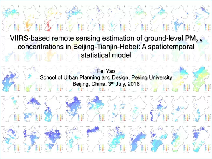
VIIRS-based remote sensing estimation of ground-level PM 2.5 concentrations in Beijing-Tianjin-Hebei: A spatiotemporal statistical model Fei Yao School of Urban Planning and Design, Peking University Beijing, China. 3 rd July, 2016

Contents Part I Introduction Part II Data & Methods Part III Results Part IV Discussion Part V Conclusions

Contents Part I Introduction Part II Data & Methods Part III Results Part IV Discussion Part V Conclusions

Part One Introduction What is PM 2.5 ?  Particles with aerodynamic diameters of less than 2.5 μm Source: US MA

Part One Introduction Adverse outcomes associated with PM 2.5  Decreasing the visibility of the atmosphere (Tao et al. 2007; Liu et al. 2013) Source: Sina Weibo

Part One Introduction Adverse outcomes associated with PM 2.5  Increasing cardiovascular- and respiratory-related morbidity and mortality (Pope et al. 2002; Dominici et al. 2006; Pope and Dockery 2006) Source: http://www.healthdata.org/china

Part One Introduction The significance of PM 2.5 data collection  Conducting environmental epidemiologic studies  Drafting appropriate air pollution control polices

Part One Introduction Two ways for PM 2.5 data collection  Ground monitoring Expensive operating costs Uneven spatial distribution of monitoring sites No temporally- and spatially- full covered PM 2.5 data Source: http://113.108.142.147:20035/emcpublish/

Part One Introduction Two ways for PM 2.5 data collection  Using satellite-derived aerosol optical depth (AOD) to estimate  Temporally- and spatially- full covered PM 2.5 data collection is possible Retrieval Spatial Lastest Sensor Satellite Remarks algorithm resolution version 10km DT C6 C5 has been applied mostly 3km(C6) MODIS Terra/Aqua The accuracy of C6 is much higher DB 10km C6 than C5 MAIAC 1km trial version Not yet global coverage High prediction accuracy, however, MISR Terra EOF 17.6km V22 long revisit period. Ended in Octobor, 2010 because of SeaWiFS SeaStar DB 13.5km V004 a mechanical trouble An explanation and improvement of VIIRS Suomi-NPP DT 6km/750m beta version AVHRR and MODIS

Part One Introduction Two limitations of previous satellite related studies  Previous studies used MODIS C5 and MISR AOD data mostly, however, their spatial resolutions are relatively coarse Retrieval Spatial Lastest Sensor Satellite Remarks algorithm resolution version 10km DT C6 C5 has been applied mostly 3km(C6) MODIS Terra/Aqua The accuracy of C6 is much higher DB 10km C6 than C5 MAIAC 1km trial version Not yet global coverage High prediction accuracy, however, MISR Terra EOF 17.6km V22 long revisit period. Ended in Octobor, 2010 because of SeaWiFS SeaStar DB 13.5km V004 a mechanical trouble An explanation and improvement of VIIRS Suomi-NPP DT 6km/750m beta version AVHRR and MODIS  We will explore the performance of VIIRS AOD

Part One Introduction Two limitations of previous satellite related studies  Quantitative relationships between PM 2.5 and AOD were built using statistical models mostly, however, these models rarely simultaneously considered the temporal and spatial variations of PM 2.5 -AOD relationships Temporal variations Spatial variations Statistical Models Representatives considered considered Simple linear model Engel-Cox et al. 2004 No No Multiple linear regression model Jia et al. 2014 No No Liu et al. 2005 Generalized linear regression model No No Liu et al. 2007 Hu et al. 2013 Geographically weighted regression model Song et al. 2014 No Yes Ma et al. 2014 Linear mixed effects model Li et al. 2015 Yes No Generalized additive model Liu et al. 2009 Yes Yes Hu et al. 2014 Two-stage model Yes Yes Ma et al. 2016  We will develop a spatiotemporal statistical model

Contents Part I Introduction Part II Data & Methods Part III Results Part IV Discussion Part V Conclusions

Part Two Data & Methods Data  All the data were collected from the Internet Spatial Data Type Source resolutions http://113.108.142.147:20035/emcpublish/ PM 2.5 Point \ http://zx.bjmemc.com.cn/ VIIRS AOD Raster 6 km http://www.class.ngdc.noaa.gov/saa/products/welcome Surface meteorolgical data Point \ http://www.escience.gov.cn/metdata/page/index.html Aerological data RH 1.25 ° × 1.25 ° http://disc.sci.gsfc.nasa.gov/daac- Raster bin/FTPSubset.pl?LOOKUPID_List=MAI3CPASM PBLH 0.5 ° × 0.5 ° Satellite-derived NDVI Raster 250 m https://ladsweb.nascom.nasa.gov/data/search.html Satellite derived NO 2 Raster 0.25 ° × 0.25 ° http://www.temis.nl/airpollution/no2col/no2regioomi_v2.php

Part Two Data & Methods Data integration  Nearest neighbor approach Y X PM 2.5 AOD TP SRH RF PBLH RH_PBLH NDVI NO 2 TOE TOS TOW TON seq site Time Space  We finally obtained a spatial panel dataset

Part Two Data & Methods Model development  Stage I: Time fixed effects regression model ○ 𝑄𝑁 2.5,𝑡𝑢 = 𝐽𝑜𝑢𝑓𝑠𝑑𝑓𝑞𝑢 𝑢 + β AOD ∗ AOD st + β TP ∗ TP st + β 𝑇𝑆𝐼 ∗ 𝑇𝑆𝐼 𝑡𝑢 + β 𝑆𝐺 ∗ 𝑆𝐺 𝑡𝑢 + β 𝑄𝐶𝑀𝐼 ∗ 𝑄𝐶𝑀𝐼 𝑡𝑢 + β 𝑆𝐼 𝑄𝐶𝑀𝐼 ∗ 𝑆𝐼 𝑄𝐶𝑀𝐼𝑡𝑢 + β 𝑂𝐸𝑊𝐽 ∗ 𝑂𝐸𝑊𝐽 𝑡𝑢 + β 𝑂𝑃2 𝑀𝑏𝑕 ∗ 𝑂𝑃2 𝑀𝑏𝑕𝑡𝑢 + β 𝑈𝑃𝐹 ∗ 𝑈𝑃𝐹 𝑡𝑢 + β 𝑈𝑃𝑇 ∗ 𝑈𝑃𝑇 𝑡𝑢 + β 𝑈𝑃𝑋 ∗ 𝑈𝑃𝑋 𝑡𝑢 + β 𝑈𝑃𝑂 ∗ 𝑈𝑃𝑂 𝑡𝑢 + ε 𝑡𝑢  Stage II: Geographically weighted regression model ○ 𝑆𝑓𝑡𝑗𝑒𝑣𝑏𝑚 𝑡𝑡′ = β 0,s + β AOD,𝑡 ∗ 𝐵𝑃𝐸 𝑡𝑡 ′ + ε 𝑡𝑡′ Spatial variations Temporal variations

Part Two Data & Methods Model development  Stage I: Time fixed effects regression model ○ 𝑄𝑁 2.5,𝑡𝑢 = 𝐽𝑜𝑢𝑓𝑠𝑑𝑓𝑞𝑢 𝑢 + β AOD ∗ AOD st + β TP ∗ TP st + β 𝑇𝑆𝐼 ∗ 𝑇𝑆𝐼 𝑡𝑢 + β 𝑆𝐺 ∗ 𝑆𝐺 𝑡𝑢 + β 𝑄𝐶𝑀𝐼 ∗ 𝑄𝐶𝑀𝐼 𝑡𝑢 + β 𝑆𝐼 𝑄𝐶𝑀𝐼 ∗ 𝑆𝐼 𝑄𝐶𝑀𝐼𝑡𝑢 + β 𝑂𝐸𝑊𝐽 ∗ 𝑂𝐸𝑊𝐽 𝑡𝑢 + β 𝑂𝑃2 𝑀𝑏𝑕 ∗ 𝑂𝑃2 𝑀𝑏𝑕𝑡𝑢 + β 𝑈𝑃𝐹 ∗ 𝑈𝑃𝐹 𝑡𝑢 + β 𝑈𝑃𝑇 ∗ 𝑈𝑃𝑇 𝑡𝑢 + β 𝑈𝑃𝑋 ∗ 𝑈𝑃𝑋 𝑡𝑢 + β 𝑈𝑃𝑂 ∗ 𝑈𝑃𝑂 𝑡𝑢 + ε 𝑡𝑢  Stage II: Geographically weighted regression model ○ 𝑆𝑓𝑡𝑗𝑒𝑣𝑏𝑚 𝑡𝑡′ = β 0,s + β AOD,𝑡 ∗ 𝐵𝑃𝐸 𝑡𝑡 ′ + ε 𝑡𝑡′ Spatial variations Temporal variations  Final PM 2.5 =PM 2.5 from Stage I + Residual from Stage II

Part Two Data & Methods Model validation  Statistical indicators ○ Coefficient of determination (R 2 ) ○ Mean predication error (MPE) Root-mean-square error (RMSE ) ○ ○ Residual spatial autocorrelation (Moran’s I)  Ten-folder cross validation ○ 1 ○ 2 … ○ 10 Model training Model testing

Contents Part I Introduction Part II Data & Methods Part III Results Part IV Discussion Part V Conclusions

Part Three Results Descriptive statistics Log-normally distributed Normally distributed

Part Three Results Model fitting – Time fixed effects regression model Time fixed effects regression model b P-value Magnitude Intercept* 40.813 0.000 AOD(unitless) 26.499 0.000 50.778 TP(0.1℃) 0.514 0.000 213.919 SRH(%) 1.059 0.000 82.632 RF(0.1mm) -0.048 0.003 -33.498 PBLH(m) -0.004 0.004 -13.951 RH_PBLH(%) -28.165 0.000 -21.421 NDVI(unitless) -5.910 0.051 -4.843 NO 2 _Lag 0.123 0.098 10.195 (10 15 molec/cm 2 ) TOE(0.1m/s)** -0.078 0.267 -3.651 TOS(0.1m/s) -0.414 0.000 -23.582 TOW(0.1m/s) -0.228 0.007 -9.903 TON(0.1m/s) -0.215 0.005 -8.546 * Intercept of the first day ** Not significant

Part Three Results Model fitting – Geographically weighted regression model

Part Three Results Model validation – Overfitting degree R 2 decreased by 0.03883 R 2 decreased by 0.16412

Part Three Results Model validation – Residual spatial autocorrelation

Part Three Results Predication maps of PM 2.5 concentrations  Daily estimations

Stage II Stage I Part Three Results Predication maps of PM 2.5 concentrations  Seasonal and annual averages

Part Three Results Predication maps of PM 2.5 concentrations  Cross-section analysis Major differences

Part Three Results Predication maps of PM 2.5 concentrations  PM 2.5 concentrations among all prefecture-level cities  Beijing and Tianjin were in medium level

Contents Part I Introduction Part II Data & Methods Part III Results Part IV Discussion Part V Conclusions

Part Four Discussion The novelty of methodology  Previous two-stage models often employed linear mixed effects model in their first stage while we employed time fixed effects regression model, which is computationally lighter and operationally easier for model calibration and prediction. And the model’s performance was comparable or even better.

Part Four Discussion The comparison of pollution pattern with previous studies  VIIRS AOD along with the spatiotemporal model provide much more fine spatial details on fine particle pollution in Beijing-Tianjin-Hebei