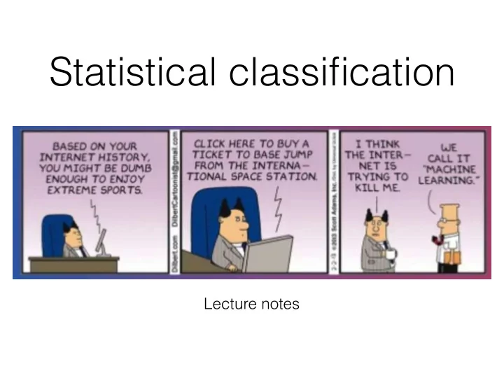
Statistical classification Lecture notes Naive Bayes Bayes' - PowerPoint PPT Presentation

Statistical classification Lecture notes

Naive Bayes

Bayes' theorem P ( c|a ) P ( a ) = P ( a|c ) P (c) P ( c|f ) – % of class c given feature(s) a – Posterior This will be our target P ( f|c ) – % of feature f given class c – Likelihood Based on data P ( c ) – % of class c in data – Class prior P ( f ) – % of feature f in data – Predictor prior Normaliser, can usually be ignored (when comparing)

Naive Bayes Based on Bayes theorem Simple, fast, easy to train Outperforms many more sophisticated algorithms BUT : It assumes every feature is independent (still surprisingly good) This is where the naivety of the method comes in! Example: Person with flu; running nose and fever are not related Big discussions on how to fix this Applications: Face recognition, Spam detection, text classification, ….

Multiple features What if more than one feature? Assume all features are independent, so that: P ( f | c ) = P (f 1 | c ) * P ( f 2 | c ) * P ( f 3 | c ) * …. * P ( f n | c ) In the previous example we could add taste, colour…

Example #1 – Fruits Class Long Sweet Yellow Banana 400 350 450 Orange 0 150 300 Other 100 150 50 P (c | long,sweet,yellow) P(long | c) * P(sweet | c) * P(yellow | c) * P (c) P(banana | long,sweet,yellow) 0.8 * 0.7 * 0.9 * 0.5 = 0.252 P(orange | long,sweet,yellow) 0.0 * 0.5 * 1.0 * 0.3 = 0.0 P(other | long,sweet,yellow) 0.5 * 0.75 * 0.25 * 0.2 = 0.01875

Example #2 – Numerical Probabilistic classifier based on fruit length Length Class 6.8 cm Banana 5.4 cm Banana 6.3 cm Banana 6.1 cm Banana 5.8 cm Banana 6.0 cm Banana 5.5 cm Banana 4.1 cm Other 4.3 cm Other 4.6 cm Other 5.1 cm Other 4.6 cm Other 4.7 cm Other 4.8 cm Other

Example #2 – Numerical Consider numerical for length Length Other Banana

Example #2 – Numerical Consider data with nose length – Two groups Length Other Banana

Example #2 – Numerical New data point Length Other Banana

Gaussian distribution Calculate means and standard deviations New values from Gaussian Probability Density Function banana other Total = 6.0 cm 4.6 cm 5.3 cm = 0.45 0.30 0.79 P (banana | L=5.4) P( pdf[5.4] | banana) * P( banana ) = 0.18 P (other | L=5.4) P( pdf[5.4] | other) * P( other ) = 0.019 Note Remove outliers > 3-4 standard devs. from mean Other functions can also be used

Genetic algorithm

Theory of evolution Evolutionary computing inspired by the evolution theory Similarly solutions are evolved Exceptional at navigating huge search spaces Fitness is measure to select new solutions (offspring) Fit offspring have better chances to “reproduce”

Representing data Genetic information is encoded in binary format Originally solutions were shown as binaries So floats, strings and more had to be converted Characters can be represented by a 4-bit string Floats can be normalised, cut to X digits, and changed into bits

Iterative process Initialise first population Calculate fitness of each solution Selection – Best solutions kept Crossover – Create new solution from best solutions Mutation – Add random variations in solutions (with a very low probability) Repeated until termination condition

Initial population Initialise population Good initial population = better solutions Most commonly they are random Initial guesses may also be used The keyword is diversity Many metrics exist to evaluate this: •Grefenstette bias •Gene-level entropy •Chromosome-Level Neighborhood Metric •Population-Level Center of Mass etc.

Fitness Fitness calculation Individual fitness compared to avg. Fitness can be based on: Fit to data/target Complexity Computation time basically anything (fitting your problem)

“Breeding" / Crossover Parents can be selected : Randomly Roulette wheel Swap genes between parents: 1-point or 2-point: Probabilistic based on fitness Uniform/half-uniform: Selected on gene level (also: three-parents crossover) Mutation swap genes values, but with a very low probability Termination criteria: Certain fitness of best “parents”

Example – Monkeys Let’s consider the infinite monkey theorem But simplified, let’s make it write “data” Initial population of 3: “lync" “deyi" and “kama" Fitness 0 1 2 Crossover could give us: “lyyi" “dama" “kamc" etc… Fitness 0 3 1 and so on until we have our data, or a particular fitness

Example – Real numbers Evaluate x to find lowest point of f(x) = 3x – x^2/10 Fitness: compare model to observations Crossover: select random BETA = [0,1], parents n,m x'1 = (1-BETA)x_m + (BETA)x_m x'2 = (1-BETA)x_n + (BETA)x_n for multi-dimensional: select one feature (x,y,z…. at random), and change only that, keep the others static Mutation : Replace parameter at random from [0,31] (low probability)

Decision trees

Decision trees Fast to train, easy to evaluate Splits data into increasingly smaller subsets in tree structure Boolean logic tracing through tree Consider it an extensive version of the game 20 Questions Also: Classification Trees & Regression trees Some similarities, but also differences, such as splitting method In regression, standard deviation is minimised to choose split

Decision trees Advantages: Very easy to visualise results Simple to understand and use Handles both numerical and categorical data … and both small and large data Disadvantages: Small changes can severely effect results Tend to not be as accurate as other methods Many-leveled categorical variables favoured higher

Example – Gotham Compile a list of some “random” people in Gotham for Santa Sex Mask Cape Tie Smokes Class Batman M Yes Yes No No Good Robin M Yes Yes No No Good Alfred M No No Yes No Good Penguin M No No Yes Yes Bad The Joker M No No Yes No Bad Harley Quinn F No No No No Bad

Example – Gotham We can create an example tree like this, skipping some features

Example – Gotham We can create an example tree like this, skipping some features How can we make it better? Pretty sure he is bad!

Building up a Decision Tree Top-most node corresponds to best predictor Too many features – too complex tree structure (Overfit) Too few features – might not even fit data (like in example) Occam’s razor: The more assumptions you make, the more unlikely the explanation => As simple as possible, but not simpler

Building up a Decision Tree Setup: Identify attribute (or value) leading to best split Create child nodes from split Recursively iterate through all child nodes until terminate

Building up a Decision Tree “Divide-and-conquer” algorithms Greedy strategies – Split based on attribute test selecting optimum, preferring homogeneous distributions With: different splitting criterion, method to reduce overfit, capable of handling incomplete, pruning, and data regression/classification Notable examples: ✦ Hunt’s algorithm (one of the earliest) ✦ ID3 – Entropy, missing values, pruning, outliers ✦ C4.5 – Entropy, missing values, error-based prune, outliers ✦ CART – Gini impurity, classification & regression, missing values, outliers ✦ Others: CHAID (chi2), MARS, SLIQ, SPRINT, …

Building up a Decision Tree Feature selected based on “purity” – fewest diff. classes For pi = Di / D where Di is # points for class i Gini impurity (CART, SLIQ, SPRINT, …) Misclassification error Measures misclassification error Error = 1 - max(pi)

Building up a Decision Tree Feature selected based on “purity” – fewest diff. classes For pi = |Di|/|D| where Di is # points in class i Entropy (ID3, C4.5, …) Compares impurity between parent and child nodes Information gain measures reduction in entropy from split Entropy(parent) - Entropy(children) [normalised ā by #/total#]

Building up a Decision Tree Binary (Yes/No, Case#1/#2, …) Nominal/Ordinal class with many values (small, medium, large) Can be binned to become binary, else no optimum split needed Continuous Numerical values such as height, temperature… Can be binary using split point (e.g. T > 100 degrees) Instead of brute force, sort and select best split point

Building up a Decision Tree But when to stop? • all nodes have same class, • all nodes have identical attribute values • Certain “depth” • if instances are independent of available features (e.g. chi2) • if further split does not improve purity • not enough data

Decision trees – Issues Tree replication problem: The same subtree can appear at different branches Irrelevant data and noise makes them unstable => Several iterations Post-processing: Prune tree to avoid overfitting, or simplify