Statistical Analysis of Corpus Data with R Word Frequency - PowerPoint PPT Presentation
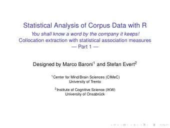
Statistical Analysis of Corpus Data with R Word Frequency Distributions: The zipfR Package Designed by Marco Baroni 1 and Stefan Evert 2 1 Center for Mind/Brain Sciences (CIMeC) University of Trento 2 Institute of Cognitive Science (IKW)
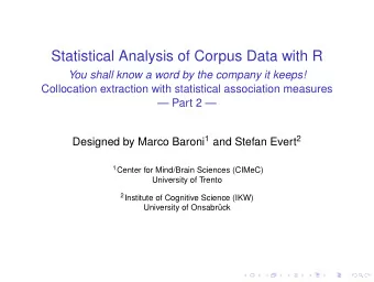
Statistical Analysis of Corpus Data with R Word Frequency Distributions: The zipfR Package Designed by Marco Baroni 1 and Stefan Evert 2 1 Center for Mind/Brain Sciences (CIMeC) University of Trento 2 Institute of Cognitive Science (IKW) University of Onsabrück
Outline Lexical statistics & word frequency distributions Basic notions of lexical statistics Typical frequency distribution patterns Zipf’s law Some applications Statistical LNRE Models ZM & fZM Sampling from a LNRE model Great expectations Parameter estimation for LNRE models zipfR
Lexical statistics Zipf 1949/1961, Baayen 2001, Evert 2004 ◮ Statistical study of the frequency distribution of types (words or other linguistic units) in texts ◮ remember the distinction between types and tokens ? ◮ Different from other categorical data because of the extreme richness of types ◮ people often speak of Zipf’s law in this context
Basic terminology ◮ N : sample / corpus size, number of tokens in the sample ◮ V : vocabulary size, number of distinct types in the sample ◮ V m : spectrum element m , number of types in the sample with frequency m (i.e. exactly m occurrences) ◮ V 1 : number of hapax legomena , types that occur only once in the sample (for hapaxes, #types = #tokens) ◮ A sample: a b b c a a b a ◮ N = 8, V = 3, V 1 = 1
Rank / frequency profile ◮ The sample: c a a b c c a c d ◮ Frequency list ordered by decreasing frequency t f c 4 a 3 b 1 d 1
Rank / frequency profile ◮ The sample: c a a b c c a c d ◮ Frequency list ordered by decreasing frequency t f c 4 a 3 b 1 d 1 ◮ Rank / frequency profile: ranks instead of type labels r f 1 4 2 3 3 1 4 1 ◮ Expresses type frequency f r as function of rank of a type
Rank/frequency profile of Brown corpus
Top and bottom ranks in the Brown corpus top frequencies bottom frequencies r f word rank range f randomly selected examples 1 62642 the 7967– 8522 10 recordings, undergone, privileges 2 35971 of 8523– 9236 9 Leonard, indulge, creativity 3 27831 and 9237–10042 8 unnatural, Lolotte, authenticity 4 25608 to 10043–11185 7 diffraction, Augusta, postpone 5 21883 a 11186–12510 6 uniformly, throttle, agglutinin 6 19474 in 12511–14369 5 Bud, Councilman, immoral 7 10292 that 14370–16938 4 verification, gleamed, groin 8 10026 is 16939–21076 3 Princes, nonspecifically, Arger 9 9887 was 21077–28701 2 blitz, pertinence, arson 10 8811 for 28702–53076 1 Salaries, Evensen, parentheses
Frequency spectrum ◮ The sample: c a a b c c a c d ◮ Frequency classes: 1 ( b , d ), 3 ( a ), 4 ( c ) ◮ Frequency spectrum: m V m 1 2 3 1 4 1
Frequency spectrum of Brown corpus 20000 15000 10000 V_m 5000 0 1 2 3 4 5 6 7 8 9 11 13 15 m
Vocabulary growth curve ◮ The sample: a b b c a a b a
Vocabulary growth curve ◮ The sample: a b b c a a b a ◮ N = 1, V = 1, V 1 = 1 ( V 2 = 0, . . . )
Vocabulary growth curve ◮ The sample: a b b c a a b a ◮ N = 1, V = 1, V 1 = 1 ( V 2 = 0, . . . ) ◮ N = 3, V = 2, V 1 = 1 ( V 2 = 1, V 3 = 0, . . . )
Vocabulary growth curve ◮ The sample: a b b c a a b a ◮ N = 1, V = 1, V 1 = 1 ( V 2 = 0, . . . ) ◮ N = 3, V = 2, V 1 = 1 ( V 2 = 1, V 3 = 0, . . . ) ◮ N = 5, V = 3, V 1 = 1 ( V 2 = 2, V 3 = 0, . . . )
Vocabulary growth curve ◮ The sample: a b b c a a b a ◮ N = 1, V = 1, V 1 = 1 ( V 2 = 0, . . . ) ◮ N = 3, V = 2, V 1 = 1 ( V 2 = 1, V 3 = 0, . . . ) ◮ N = 5, V = 3, V 1 = 1 ( V 2 = 2, V 3 = 0, . . . ) ◮ N = 8, V = 3, V 1 = 1 ( V 2 = 0, V 3 = 1, V 4 = 1, . . . )
Vocabulary growth curve of Brown corpus With V 1 growth in red (curve smoothed with binomial interpolation) 40000 30000 V and V_1 20000 10000 0 0e+00 2e+05 4e+05 6e+05 8e+05 1e+06 N
Outline Lexical statistics & word frequency distributions Basic notions of lexical statistics Typical frequency distribution patterns Zipf’s law Some applications Statistical LNRE Models ZM & fZM Sampling from a LNRE model Great expectations Parameter estimation for LNRE models zipfR
Typical frequency patterns Across text types & languages
Typical frequency patterns The Italian prefix ri- in the la Repubblica corpus
Is there a general law? ◮ Language after language, corpus after corpus, linguistic type after linguistic type, . . . we observe the same “few giants, many dwarves” pattern ◮ Similarity of plots suggests that relation between rank and frequency could be captured by a general law
Is there a general law? ◮ Language after language, corpus after corpus, linguistic type after linguistic type, . . . we observe the same “few giants, many dwarves” pattern ◮ Similarity of plots suggests that relation between rank and frequency could be captured by a general law ◮ Nature of this relation becomes clearer if we plot log f as a function of log r
Outline Lexical statistics & word frequency distributions Basic notions of lexical statistics Typical frequency distribution patterns Zipf’s law Some applications Statistical LNRE Models ZM & fZM Sampling from a LNRE model Great expectations Parameter estimation for LNRE models zipfR
Zipf’s law ◮ Straight line in double-logarithmic space corresponds to power law for original variables ◮ This leads to Zipf’s (1949, 1965) famous law: C f ( w ) = r ( w ) a
Zipf’s law ◮ Straight line in double-logarithmic space corresponds to power law for original variables ◮ This leads to Zipf’s (1949, 1965) famous law: C f ( w ) = r ( w ) a ◮ With a = 1 and C = 60,000, Zipf’s law predicts that: ◮ most frequent word occurs 60,000 times ◮ second most frequent word occurs 30,000 times ◮ third most frequent word occurs 20,000 times ◮ and there is a long tail of 80,000 words with frequencies between 1.5 and 0.5 occurrences(!)
Zipf’s law Logarithmic version ◮ Zipf’s power law: C f ( w ) = r ( w ) a ◮ If we take logarithm of both sides, we obtain: log f ( w ) = log C − a log r ( w ) ◮ Zipf’s law predicts that rank / frequency profiles are straight lines in double logarithmic space ◮ Best fit a and C can be found with least-squares method
Zipf’s law Logarithmic version ◮ Zipf’s power law: C f ( w ) = r ( w ) a ◮ If we take logarithm of both sides, we obtain: log f ( w ) = log C − a log r ( w ) ◮ Zipf’s law predicts that rank / frequency profiles are straight lines in double logarithmic space ◮ Best fit a and C can be found with least-squares method ◮ Provides intuitive interpretation of a and C : ◮ a is slope determining how fast log frequency decreases ◮ log C is intercept , i.e., predicted log frequency of word with rank 1 (log rank 0) = most frequent word
Zipf’s law Fitting the Brown rank/frequency profile
Zipf-Mandelbrot law Mandelbrot 1953 ◮ Mandelbrot’s extra parameter: C f ( w ) = ( r ( w ) + b ) a ◮ Zipf’s law is special case with b = 0 ◮ Assuming a = 1, C = 60,000, b = 1: ◮ For word with rank 1, Zipf’s law predicts frequency of 60,000; Mandelbrot’s variation predicts frequency of 30,000 ◮ For word with rank 1,000, Zipf’s law predicts frequency of 60; Mandelbrot’s variation predicts frequency of 59.94 ◮ Zipf-Mandelbrot law forms basis of statistical LNRE models ◮ ZM law derived mathematically as limiting distribution of vocabulary generated by a character-level Markov process
Zipf-Mandelbrot vs. Zipf’s law Fitting the Brown rank/frequency profile
Outline Lexical statistics & word frequency distributions Basic notions of lexical statistics Typical frequency distribution patterns Zipf’s law Some applications Statistical LNRE Models ZM & fZM Sampling from a LNRE model Great expectations Parameter estimation for LNRE models zipfR
Applications of word frequency distributions ◮ Most important application: extrapolation of vocabulary size and frequency spectrum to larger sample sizes ◮ productivity (in morphology, syntax, . . . ) ◮ lexical richness (in stylometry, language acquisition, clinical linguistics, . . . ) ◮ practical NLP (est. proportion of OOV words, typos, . . . ) ☞ need method for predicting vocab. growth on unseen data
Applications of word frequency distributions ◮ Most important application: extrapolation of vocabulary size and frequency spectrum to larger sample sizes ◮ productivity (in morphology, syntax, . . . ) ◮ lexical richness (in stylometry, language acquisition, clinical linguistics, . . . ) ◮ practical NLP (est. proportion of OOV words, typos, . . . ) ☞ need method for predicting vocab. growth on unseen data ◮ Direct applications of Zipf’s law ◮ population model for Good-Turing smoothing ◮ realistic prior for Bayesian language modelling ☞ need model of type probability distribution in the population
Vocabulary growth: Pronouns vs. ri- in Italian N V (pron.) V ( ri- ) 5000 67 224 10000 69 271 15000 69 288 20000 70 300 25000 70 322 30000 71 347 35000 71 364 40000 71 377 45000 71 386 50000 71 400 . . . . . . . . .
Vocabulary growth: Pronouns vs. ri- in Italian Vocabulary growth curves 80 1000 60 800 V and V_1 V and V_1 600 40 400 20 200 0 0 0 2000 4000 6000 8000 10000 0 200000 600000 1000000 N N
Recommend
More recommend
Explore More Topics
Stay informed with curated content and fresh updates.
