STABILITY ISSUES IN PEAK LIMITING CURRENT MODE CONTROLLED BUCK - PowerPoint PPT Presentation

STABILITY ISSUES IN PEAK LIMITING CURRENT MODE CONTROLLED BUCK CONVERTER Marija Glišić, Predrag Pejović

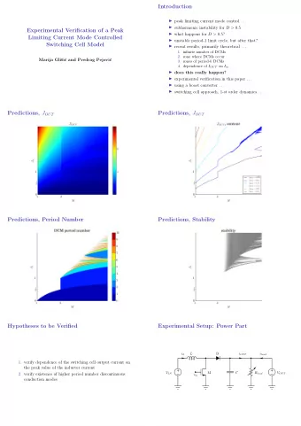
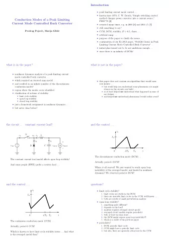
Introduction ◮ peak limiting current mode control . . . ◮ known since 1978, C. W. Deisch, “Simple switching control method changes power converter into a current source,” PESC’78 [2] ◮ revisited many times, e.g. in 2001 [6] and 2011 (!) [7] ◮ still something to say? ◮ CCM, DCM, stability, D > 0 . 5 , chaos, . . . ◮ artificial ramp . . . ◮ purpose of the paper to clarify the issues . . . ◮ and this presentation contains more than the paper does!

the circuit . . . constant current load! S i S v X i L L i D i C + + v IN D C i OUT v OUT − −

the waveform, . . . DCM assumed! i L I m 0 d T S T S t i L = f S L v IN 1 I 2 m 2 v OUT v IN − v OUT

decoupling, switching cell . . . also assumed, implicitly! S i S v X i L L i D + + v IN D v OUT − − used to draw i L , to compute i L . . . v OUT assumed constant over T S . . . implicitly!

decoupling, averaged model . . . v L i S i L + − i D i C + + v IN C i OUT v OUT − −

decoupling, averaged model simplified . . . i C + i L C i OUT v OUT − C d v OUT = i L − i OUT d t and i L is given three slides above . . . and our story begins here . . .

Averaging C d v OUT = f S L v IN 1 I 2 − i OUT m d t 2 v OUT v IN − v OUT overline notation consistent? d v OUT = 0 fixed points ⇒ d t two fixed points . . . (overline notation dropped) � v 2 − f S L I 2 v OUT 1 , 2 = v IN m v IN IN ± 2 4 2 i OUT and it is not a good practice to have two when you need only one . . .

an example . . . v IN = 12 V, f S = 100 kHz, L = 36 µ H, I m = 0 . 5 A, i OUT = 0 . 2 A, C = 200 µ F i L = 0 . 45 A 12 V 1 v OUT 12 V − v OUT i L = i OUT = 0 . 2 A  3 V  fixed points: v OUT =  9 V

fixed points . . . I m = 0 . 5 A 0 . 50 0 . 45 0 . 40 0 . 35 i L , i OUT [ A ] 0 . 30 0 . 25 0 . 20 0 . 15 0 . 10 0 . 05 0 . 00 0 1 2 3 4 5 6 7 8 9 10 11 12 v OUT [ V ]

detour: normalization m X � v X v IN j Y � f S L i Y v IN τ � t = f S t T S result: L d i L d j L d t = v L d τ = m L ⇒ special: v IN ⇒ 1 , v OUT ⇒ M , I m ⇒ J m , i OUT ⇒ j OUT

fixed points, normalized V base = 12 V, I base = 10 3 A J m = 0 . 15 , j OUT = 0 . 06 � M 1 , 2 = 1 1 J 2 m 2 ± 4 − 2 j OUT  1 / 4  fixed ponts: M =  3 / 4

fixed points . . . normalized! J m = 15 / 100 15 / 100 12 / 100 9 / 100 j L , j OUT 6 / 100 3 / 100 0 0 1 1 / 4 1 / 2 3 / 4 M

Linearization C d v OUT = f S L v IN 1 I 2 m d t 2 v OUT v IN − v OUT v OUT + α m � I m − � s C � v OUT = g IN � v IN + g OUT � i OUT f S L I 2 g IN = ∂ i L M = − 2 ( V IN − V OUT ) 2 ∂ v IN = f S L I 2 ∂ i L M V IN (2 V OUT − V IN ) g OUT = OUT ( V IN − V OUT ) 2 ∂ v OUT 2 V 2 α m = ∂ i L f S L I M V IN = V OUT ( V IN − V OUT ) ∂ I m

transfer functions . . . v IN + H m � I m − H OUT � � v OUT = H IN � i OUT g IN H IN = s C − g OUT α m H m = s C − g OUT 1 H OUT = s C − g OUT ∂ i L stability: g OUT < 0 , < 0 ∂ v OUT . . . previous slide: 2 V OUT − V IN < 0 , V OUT < V IN / 2

fixed points, once again . . . what’s going on? I m = 0 . 5 A 0 . 50 0 . 45 0 . 40 0 . 35 i L , i OUT [ A ] 0 . 30 0 . 25 0 . 20 0 . 15 0 . 10 0 . 05 0 . 00 0 1 2 3 4 5 6 7 8 9 10 11 12 v OUT [ V ]

Discrete Time Model S i S v X i L L i D + + v IN D v OUT − − ◮ v OUT assumed constant over T S ◮ want to know mapping i L (0) → i L ( T S ) . . . knowing I m , v IN , v OUT , f S , L . . . . . . or just J m and M ? ( 5 → 2 ) � n T S 1 ◮ i L ( n ) � ( n − 1) T S i L ( t ) dt is an auxiliary (but important!) T S result ◮ normalization is useful here!!!

normalization, three cases . . . d j L ◮ S-on, D-off: dt = 1 − M d j L ◮ S-off, D-on: dt = − M d j L ◮ S-off, D-off: dt = 0 But only two parameters, J m and M ! Look for j L ( n − 1) → j L ( n ) and j L ( n ) !

three cases, again . . . case 1, no switching interval j L J m j L (1) j L (0) 0 1 τ

three cases, again . . . case 2, continuous conduction interval j L J m j L (1) j L (0) 0 τ 1 1 τ

three cases, again . . . case 3, discontinuous conduction interval j L J m j L (0) j L (1) = 0 0 τ 1 1 τ τ 1 + τ 2

analytical . . .   1 − M + j L (0) ,     if     j L (0) < J m + M − 1        1 M    1 − M J m − M − 1 − M j L (0) ,      if   J m + M − 1 < j L (0) j L (1) ( j L (0) , M, J m ) =  and     j L (0) < J m   M + M − 1           0 ,     if    J m   M + M − 1 < j L (0) . . . similar for j OUT . . .

Basins of Attraction I m = 0 . 5 A 0 . 50 0 . 45 0 . 40 0 . 35 i L , i OUT [ A ] 0 . 30 0 . 25 0 . 20 0 . 15 0 . 10 0 . 05 0 . 00 0 1 2 3 4 5 6 7 8 9 10 11 12 v OUT [ V ]

trajectory of v OUT . . . 12 10 8 v OUT [ V ] 6 4 v OUT (0) = 9 . 1 V 2 v OUT (0) = 8 . 9 V 0 0 10 20 30 40 50 t [ ms ]

trajectory of i L . . . v OUT (0) = 9 . 1 V v OUT (0) = 8 . 9 V 0 . 25 i L [ A ] 0 . 20 0 . 15 0 . 10 0 10 20 30 40 50 t [ ms ]

steady state waveform of i L , . . . “twin peaks” v OUT = 10 . 123190 V ; I m = 0 . 5 A ; I OUT = 0 . 2 A 0 . 5 0 . 4 0 . 3 i L [ A ] 0 . 2 0 . 1 0 . 0 − 0 . 1 0 5 10 15 20 t [ µ s ]

actually happens . . . 1 . 2 1 . 0 0 . 8 0 . 6 i L [ A ] 0 . 4 0 . 2 0 . 0 − 0 . 2 − 0 . 4 0 5 10 15 20 25 30 35 40 45 50 t [ µ s ]

Limit Cycles ◮ the problem begins when the converter would enter CCM for D > 1 / 2 ◮ supposed limit cycle is unstable! ◮ but the converter operates in a stable limit cycle, regardless our assumptions . . . ◮ . . . it happened to be period-2 DCM . . . ◮ . . . and here the mess starts . . .

supposed . . . I m = 0 . 5 A 0 . 50 0 . 45 0 . 40 0 . 35 i L , i OUT [ A ] 0 . 30 0 . 25 0 . 20 0 . 15 0 . 10 0 . 05 0 . 00 0 1 2 3 4 5 6 7 8 9 10 11 12 v OUT [ V ]

actual . . . I m = 0 . 5 A 0 . 50 0 . 45 0 . 40 0 . 35 i L , i OUT [ A ] 0 . 30 0 . 25 0 . 20 0 . 15 0 . 10 0 . 05 0 . 00 0 1 2 3 4 5 6 7 8 9 10 11 12 v OUT [ V ]

and we have it analytical . . . in the paper! (boring) 0 . 5 0 . 4 0 . 3 i L [ A ] 0 . 2 0 . 1 0 . 0 10 . 0 10 . 5 11 . 0 11 . 5 12 . 0 v OUT [ V ]

iterate over J m . . . not in the paper!

iterate over J m . . . not in the paper!

important: operating mode chart . . . not in the paper! period- n CCM 1 period-1 CCM J m period- n DCM 1 / 2 1 / 4 period-1 DCM 0 0 1 1 / 2 M

iterate over J m . . . not in the paper!

iterate over J m . . . not in the paper!

DCM, period number, n = 1 , not in the paper!

DCM, period number, n = 2 , not in the paper!

DCM, period number, n = 3 , not in the paper!

DCM, period number, n = 4 , not in the paper!

DCM, period number, n = 5 , not in the paper!

DCM, period number, n = 6 , not in the paper!

DCM, period number, n = 7 , not in the paper!

DCM, period number, n = 8 , not in the paper!

DCM, period number, n = 9 , not in the paper!

DCM, period number, n = 10 , not in the paper!

period number, in color, . . . not in the paper!

stability . . . not in the paper!

Conclusions, 1 ◮ buck converter analyzed, PLCMC applied ◮ decoupling (in reversed order): 1. “averaged” model, linearized later on . . . 2. “discrete time” model ◮ stability: 1. stability of the averaged model 2. limit cycle stability (stability of the discrete time model) ◮ limit cycle instability: 1. occurs in would-be CCM for D > 1 / 2 2. results in sensitive small-signal parameters 3. affects averaged model stability! ◮ analytical techniques, models, normalization . . .

Conclusions, 2 ◮ in the paper , case study for J m = 0 . 15 ◮ analytical techniques developed, discrete time model ◮ detailed study of the discrete time model ◮ identification of modes ◮ pretty good analytical description . . . ◮ analysis of stability

Conclusions, 3 ◮ in this presentation , generalized over J m , the remaining degree of freedom, along with M , completeness achieved ◮ important: 1. occurrence of period- n modes when assumed period-1 CCM has unstable limit cycle, for D > 1 / 2 2. both period- n CCM and period- n DCM exist ◮ charts: 1. chart of modes 2. chart of periodicity (chart of n ) 3. chart of stability

Conclusion avoid period- n modes!