Spectral properties of Google matrix Klaus Frahm Quantware MIPS - PowerPoint PPT Presentation

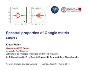
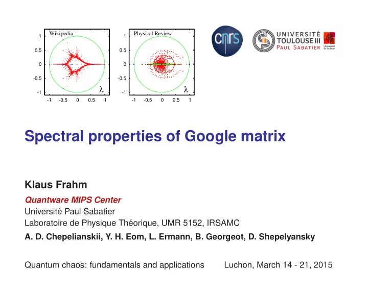
Wikipedia Physical Review 1 1 0.5 0.5 0 0 -0.5 -0.5 λ λ -1 -1 -1 -0.5 0 0.5 1 -1 -0.5 0 0.5 1 Spectral properties of Google matrix Klaus Frahm Quantware MIPS Center Universit´ e Paul Sabatier Laboratoire de Physique Th´ eorique, UMR 5152, IRSAMC A. D. Chepelianskii, Y. H. Eom, L. Ermann, B. Georgeot, D. Shepelyansky Quantum chaos: fundamentals and applications Luchon, March 14 - 21, 2015

Contents Perron-Frobenius operators . . . . . . . . . . . . . . . . . 3 PF Operators for directed networks . . . . . . . . . . . . . . 4 PageRank . . . . . . . . . . . . . . . . . . . . . . . . . . 6 Numerical diagonalization . . . . . . . . . . . . . . . . . . 7 University Networks . . . . . . . . . . . . . . . . . . . . . 9 Wikipedia . . . . . . . . . . . . . . . . . . . . . . . . . . . 12 Twitter network . . . . . . . . . . . . . . . . . . . . . . . . 14 Random Perron-Frobenius matrices . . . . . . . . . . . . . 16 Poisson statistics of PageRank . . . . . . . . . . . . . . . . 18 Physical Review network . . . . . . . . . . . . . . . . . . . 20 Perron-Frobenius matrix for chaotic maps . . . . . . . . . . 26 References . . . . . . . . . . . . . . . . . . . . . . . . . . 35 2

Perron-Frobenius operators Consider a physical system with N states i = 1 , . . . , N and probabilities p i ( t ) ≥ 0 evolving by a discrete Markov process : � � p i ( t + 1) = G ij p j ( t ) with G ij = 1 , G ij ≥ 0 . j i The transition probabilities G ij provide a Perron-Frobenius matrix. Conservation of probability: � i p i ( t + 1) = � i p i ( t ) = 1 . In general G T � = G and eigenvalues λ may be complex and obey | λ | ≤ 1 . The vector e T = (1 , . . . , 1) is left eigenvector with λ 1 = 1 ⇒ existence of (at least) one right eigenvector P for λ 1 = 1 also called PageRank in the context of Google matrices: G P = 1 P For non-degenerate λ 1 and finite gap | λ 2 | < 1 : t →∞ p ( t ) = P lim ⇒ Power method to compute P with rate of convergence ∼ | λ 2 | t . 3

PF Operators for directed networks Consider a directed network with N nodes 1 , . . . , N and N ℓ links. Adjacency matrix: A jk = 1 if there is a link k → j and A jk = 0 otherwise. Sum-normalization of each non-zero column of A ⇒ S 0 . Replacing each zero column ( dangling nodes ) with e/N ⇒ S . Eventually apply the damping factor α < 1 (typically α = 0 . 85 ): G ( α ) = αS + (1 − α ) 1 Google matrix: N ee T . ⇒ λ 1 is non-degenerate and | λ 2 | ≤ α . Same procedure for inverted network: A ∗ ≡ A T where S ∗ and G ∗ are obtained in the same way from A ∗ . Note: in general: S ∗ � = S T . Leading (right) eigenvector of S ∗ or G ∗ is called CheiRank . 4

Example:   0 1 1 0 0 1 0 1 1 0     A = 0 1 0 1 0     0 0 1 0 0   0 0 0 1 0     0 1 1 0 1 1 3 0 1 3 0 0 2 2 5 1 0 1 1 1 0 1 1 1     3 0     3 3 3 5     0 1 2 0 1 0 1 2 0 1 1 S 0 = 3 0 , S =     3 5     0 0 1 0 0 1 3 0 1     3 0 0     5 0 0 0 1 0 0 0 1 1 3 0 3 5 5

PageRank Example for university networks of Cambridge 2006 and Oxford 2006 ( N ≈ 2 × 10 5 and N ℓ ≈ 2 × 10 6 ). 10 -2 10 -2 PageRank Cambridge PageRank Oxford 10 -3 10 -3 α =0.85 α =0.85 CheiRank CheiRank P, P * 10 -4 P, P * 10 -4 10 -5 10 -5 10 -6 10 -6 10 0 10 1 10 2 10 3 10 4 10 5 10 0 10 1 10 2 10 3 10 4 10 5 K, K * K, K * � P ( i ) = G ij P ( j ) j P ( i ) represents the “importance” of “node/page i ” obtained as sum of all other pages j pointing to i with weight P ( j ) . Sorting of P ( i ) ⇒ index K ( i ) for order of appearance of search results in search engines such as Google. 6

Numerical diagonalization • Power method to obtain P : rate of convergence for G ( α ) ∼ α t . • Full “exact” diagonalization ( N � 10 4 ). • Arnoldi method to determine largest n A ∼ 10 2 − 10 4 eigenvalues. Idea: write k +1 � G ξ k = H jk ξ j for k = 0 , . . . , n A − 1 j =0 where ξ k +1 is obtained from Gram-Schmidt orthogonalization of Gξ k to ξ 0 , . . . , ξ k with ξ 0 being some suitable normalized initial vector. ξ 0 , . . . , ξ n A − 1 span a Krylov space of dimension n A and the eigenvalues of the “small” representation matrix H jk are (very) good approximations to the largest eigenvalues of G . Example for Twitter network of 2009: N ≈ 4 × 10 7 and N ℓ ≈ 1 . 5 × 10 9 with n A = 640 (lower N in other examples allows for higher n A ) . 7

• Practical problems due to invariant subspaces of nodes in realistic WWW networks creating large degeneracies of λ 1 (or λ 2 if α < 1 ). Decomposition in subspaces and a core space � � S ss S sc ⇒ S = 0 S cc where S ss is block diagonal according to the subspaces. The subspace blocks of S ss are all matrices of PF type with at least one eigenvalue λ 1 = 1 explaining the high degeneracies. To determine the spectrum of S apply exact (or Arnoldi) diagonalization on each subspace and the Arnoldi method to S cc to determine the largest core space eigenvalues λ j (note: | λ j | < 1 ). • Strange numerical problems to determine accurately “small” eigenvalues, in particular for (nearly) triangular network structure due to large Jordan-blocks (e.g. citation network of Physical Review). 8

University Networks 1 1 0.5 0.5 Cambridge 2006 (left), 0 0 N = 212710 , N s = 48239 -0.5 -0.5 λ λ Oxford 2006 (right), -1 -1 N = 200823 , N s = 30579 -1 -0.5 0 0.5 1 -1 -0.5 0 0.5 1 1 1 Spectrum of S (upper panels), S ∗ 0.5 0.5 (middle panels) and dependence of 0 0 rescaled level number on | λ j | (lower -0.5 -0.5 panels). λ λ -1 -1 -1 -0.5 0 0.5 1 -1 -0.5 0 0.5 1 Blue: subspace eigenvalues 0.05 0.05 0.04 Red: core space eigenvalues (with 0.04 0.03 0.03 j/N j/N Arnoldi dimension n A = 20000 ) 0.02 0.02 0.01 0.01 0 0 0.7 0.8 0.9 1 0.7 0.8 0.9 1 | λ j | | λ j | 9

PageRank for α → 1 : PageRank Cambridge PageRank Oxford 10 -2 10 -2 1- α = 0.1 1- α = 0.1 10 -4 10 -4 10 -6 10 -6 1- α = 10 -3 1- α = 10 -3 P P 10 -8 10 -8 1- α = 10 -5 1- α = 10 -5 10 -10 10 -10 1- α = 10 -7 1- α = 10 -7 10 -12 10 -12 10 0 10 1 10 2 10 3 10 4 10 5 10 0 10 1 10 2 10 3 10 4 10 5 K K 10 -1 10 -1 PageRank Cambridge PageRank Oxford 1- α = 10 -8 1- α = 10 -8 10 -3 10 -3 10 -5 10 -5 10 -1 f( α )-f(1) 10 -1 w( α ) 10 -7 10 -7 P P 10 -9 10 -4 w( α ) 10 -9 10 -4 f( α )-f(1) 10 -11 10 -11 10 -6 10 -2 10 -6 10 -2 1- α 1- α 10 -13 10 -13 10 0 10 1 10 2 10 3 10 4 10 5 10 0 10 1 10 2 10 3 10 4 10 5 K K 1 − α � � P = c j ψ j + (1 − α ) + α (1 − λ j ) c j ψ j . λ j =1 λ j � =1 � �� � subspace contributions 10

Core space gap and quasi-subspaces 1 10 -3 Cambridge 2002 Cambridge 2003 Cambridge 2004 10 -5 Cambridge 2005 10 -5 Leeds 2006 (core) (core) 10 -10 1- λ 1 ψ 1 10 -7 10 -15 10 -9 10 -20 10 3 10 4 10 5 0 100 200 300 400 K (core) N Left: Core space gap 1 − λ (core) vs N for certain british universities. 1 Red dots for gap > 10 − 9 ; blue crosses (moved up by 10 9 ) for gap < 10 − 16 . Right: first core space eigenvecteur for universities with gap < 10 − 16 or gap = 2 . 91 × 10 − 9 for Cambridge 2004. Core space gaps < 10 − 16 correspond to quasi-subspaces where it takes quite many “iterations” to reach a dangling node. 11

Wikipedia Wikipedia 2009 : N = 3282257 nodes, N ℓ = 71012307 network links. Wikipedia Wikipedia 1 1 10 -1 10 -1 Wikipedia Wikipedia 10 -3 10 -3 0.5 0.5 10 -5 10 -5 * | P, | ψ i | 10 -7 P * , | ψ i 10 -7 0 0 10 -9 10 -9 -0.5 -0.5 10 -11 10 -11 λ λ 10 -13 10 -13 -1 -1 10 0 10 1 10 2 10 3 10 4 10 5 10 6 10 0 10 1 10 2 10 3 10 4 10 5 10 6 -1 -0.5 0 0.5 1 -1 -0.5 0 0.5 1 K * , K i * K, K i Cambridge 2011 Cambridge 2011 10 -1 10 -1 Cambridge 2011 Cambridge 2011 1 1 10 -3 10 -3 10 -5 10 -5 0.5 0.5 * | P, | ψ i | 10 -7 P * , | ψ i 10 -7 0 0 10 -9 10 -9 10 -11 10 -11 -0.5 -0.5 10 -13 10 -13 λ λ 10 0 10 1 10 2 10 3 10 4 10 5 10 0 10 1 10 2 10 3 10 4 10 5 -1 -1 K * , K i * K, K i -1 -0.5 0 0.5 1 -1 -0.5 0 0.5 1 left (right): PageRank (CheiRank) black: PageRank (CheiRank) at α = 0 . 85 grey: PageRank (CheiRank) at α = 1 − 10 − 8 red and green: first two core space eigenvectors blue and pink: two eigenvectors with large imaginary part in the eigenvalue 12

“Themes” of certain Wikipedia eigenvectors: math (function, geometry,surface, logic-circuit) England poetry Iceland aircraft Kuwait poetry Bangladesh football 0.5 biology song muscle-artery muscle-artery New Zeland DNA Austria Bible Poland muscle-artery music 0 -1 -0.5 0 0.5 1 Australia Canada protein Brazil China RNA skin war rail 0 Texas-Dallas-Houston Gaafu Alif Atoll -0.82 -0.8 -0.78 -0.76 -0.74 -0.72 Quantum Leap Language Switzerland Australia Australia England mathematics 0 0.8 0.82 0.84 0.86 0.88 0.9 0.92 0.94 0.96 0.98 13

Twitter network Twitter 2009 : N = 41652230 nodes, N ℓ = 1468365182 network links. Matrix structure in K-rank order: Number N G of non-empty matrix elements in K × K -square: 1 10 3 0.8 10 2 0.6 N G /K 2 N G /K 0.4 10 1 0.2 10 0 0 10 0 10 2 10 4 10 6 10 8 0 500 1000 K K 14