Spectral properties of Google matrix Lecture 3 Klaus Frahm - PowerPoint PPT Presentation

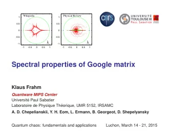
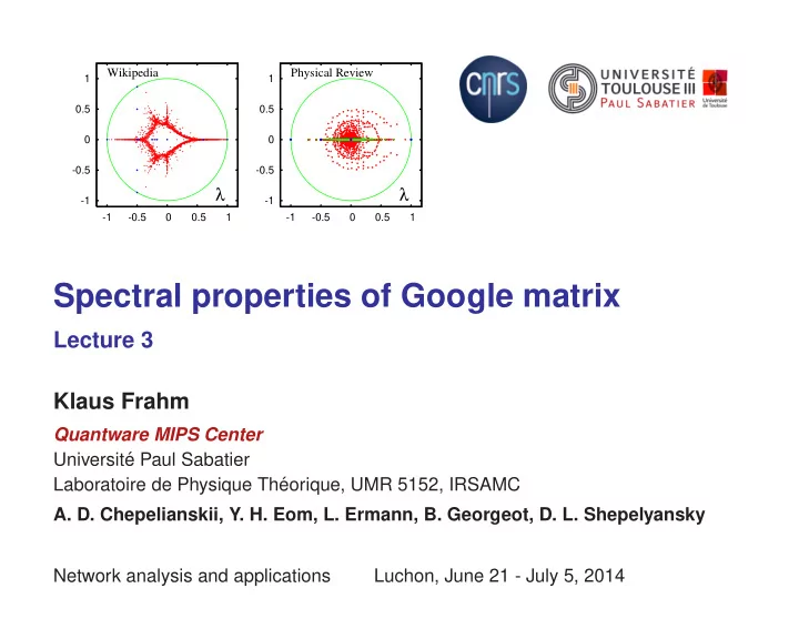
Wikipedia Physical Review 1 1 0.5 0.5 0 0 -0.5 -0.5 λ λ -1 -1 -1 -0.5 0 0.5 1 -1 -0.5 0 0.5 1 Spectral properties of Google matrix Lecture 3 Klaus Frahm Quantware MIPS Center Universit´ e Paul Sabatier Laboratoire de Physique Th´ eorique, UMR 5152, IRSAMC A. D. Chepelianskii, Y. H. Eom, L. Ermann, B. Georgeot, D. L. Shepelyansky Network analysis and applications Luchon, June 21 - July 5, 2014

Contents Random Perron-Frobenius matrices . . . . . . . . . . . . . 3 Poisson statistics of PageRank . . . . . . . . . . . . . . . . 6 Physical Review network . . . . . . . . . . . . . . . . . . . 8 Triangular approximation . . . . . . . . . . . . . . . . . . . 11 Full Physical Review network . . . . . . . . . . . . . . . . . 14 Fractal Weyl law . . . . . . . . . . . . . . . . . . . . . . . 21 ImpactRank for influence propagation . . . . . . . . . . . . 22 Integer network . . . . . . . . . . . . . . . . . . . . . . . . 23 References . . . . . . . . . . . . . . . . . . . . . . . . . . 29 2

Random Perron-Frobenius matrices Construct random matrix ensembles G ij such that: • G ij ≥ 0 • G ij are (approximately) non-correlated and distributed with the same distribution P ( G ij ) (of finite variance σ 2 ). • � j G ij = 1 ⇒ � G ij � = 1 /N • ⇒ average of G has one eigenvalue λ 1 = 1 ( ⇒ “flat” PageRank) and other eigenvalues λ j = 0 (for j � = 1 ). • degenerate perturbation theory for the fluctuations ⇒ circular √ eigenvalue density with R = Nσ and one unit eigenvalue. 3

Different variants of the model: • uniform full : P ( G ) = N/ 2 for 0 ≤ G ≤ 2 /N √ ⇒ R = 1 / 3 N • uniform sparse with Q non-zero elements per column: P ( G ) = Q/ 2 for 0 ≤ G ≤ 2 /Q with probability Q/N and G = 0 with probability 1 − Q/N R = 2 / √ 3 Q ⇒ • constant sparse with Q non-zero elements per column: G = 1 /Q with probability Q/N and G = 0 with probability 1 − Q/N R = 1 / √ Q ⇒ • powerlaw with p ( G ) = D (1 + aG ) − b for 0 ≤ G ≤ 1 and 2 < b < 3 : C ( b ) = ( b − 2) ( b − 1) / 2 � R = C ( b ) N 1 − b/ 2 b − 1 ⇒ , 3 − b 4

Numerical verification: 1 0.02 0.5 triangular 0 0 uniform full: random and -0.5 N = 400 average -0.02 λ λ -1 -0.02 0 0.02 -1 -0.5 0 0.5 1 1 1 0.5 0.5 constant sparse: uniform sparse: 0 0 N = 400 , N = 400 , -0.5 -0.5 Q = 20 Q = 20 λ λ -1 -1 -1 -0.5 0 0.5 1 -1 -0.5 0 0.5 1 1 power law: power law case: R = 0.67 N -0.22 0.5 0.2 R th ∼ N − 0 . 25 b = 2 . 5 0 R -0.5 λ -1 0.1 -1 -0.5 0 0.5 1 100 1000 N 5

Poisson statistics of PageRank 1 1 original data original data p Pois (s) p Pois (s) p Wig (s) p Wig (s) 0.8 0.8 0.6 0.6 p(s) p(s) 0.4 0.4 Twitter Wikipedia 0.2 0.2 0 0 0 1 2 3 4 0 1 2 3 4 s s Identify PageRank values to “energy-levels”: P ( i ) = exp( − E i /T ) /Z with Z = � i exp( − E i /T ) and an effective temperature T (can be choosen: T = 1 ). 6

Twitter Wikipedia 10 9.5 7.5 9 E i E i 7 8.5 8 6.5 7.5 0.8 0.85 0.9 0.8 0.85 0.9 α α 9.8 7.5 9.7 7.4 E i E i 9.6 7.3 9.5 7.2 0.8 0.85 0.9 0.8 0.85 0.9 α α Parameter dependance of E i = − ln( P i ) on the damping factor α . 7

Physical Review network N = 463347 nodes and N ℓ = 4691015 links. Coarse-grained matrix structure ( 500 × 500 cells): left: time ordered right: journal and then time ordered “11” Journals of Physical Review: (Phys. Rev. Series I), Phys. Rev., Phys. Rev. Lett., (Rev. Mod. Phys.), Phys. Rev. A, B, C, D, E, (Phys. Rev. STAB and Phys. Rev. STPER). 8

⇒ nearly triangular matrix structure of adjacency matrix: most citations links t → t ′ are for t > t ′ (“past citations”) but there is small number ( 12126 = 2 . 6 × 10 − 3 N ℓ ) of links t → t ′ with t ≤ t ′ corresponding to future citations . Spectrum by “double-precision” Arnoldi method with n A = 8000 : 1 1 0.5 0.5 0 0 -0.5 -0.5 λ λ -1 -1 -1 -0.5 0 0.5 1 -1 -0.5 0 0.5 1 Numerical problem: eigenvalues with | λ | < 0 . 3 − 0 . 4 are not reliable! Reason: large Jordan subspaces associated to the eigenvalue λ = 0 . 9

“very bad” Jordan perturbation theory: Consider a “perturbed” Jordan block of size D :   0 1 · · · 0 0 0 0 · · · 0 0   . . . . ...   . . . . . . . .     0 0 · · · 0 1   ε 0 · · · 0 0 characteristic polynomial: λ D − ( − 1) D ε ε = 0 ⇒ λ = 0 λ j = − ε 1 /D exp(2 πij/D ) ε � = 0 ⇒ for D ≈ 10 2 and ε = 10 − 16 ⇒ “Jordan-cloud” of artifical eigenvalues due to rounding errors in the region | λ | < 0 . 3 − 0 . 4 . 10

Triangular approximation Remove the small number of links due to “future citations”. Semi-analytical diagonalization is possible: S = S 0 + e d T /N where e n = 1 for all nodes n , d n = 1 for dangling nodes n and d n = 0 otherwise. S 0 is the pure link matrix which is nil-potent : S l 0 = 0 with l = 352 . Let ψ be an eigenvector of S with eigenvalue λ and C = d T ψ . • If C = 0 ⇒ ψ eigenvector of S 0 ⇒ λ = 0 since S 0 nil-potent. These eigenvectors belong to large Jordan blocks and are responsible for the numerical problems. Note: Similar situation as in network of integer numbers where l = [log 2 ( N )] and numerical instability for | λ | < 0 . 01 . 11

• If C � = 0 ⇒ λ � = 0 since the equation S 0 ψ = − C e/N does not have a solution ⇒ λ 1 − S 0 invertible. l − 1 � j � S 0 ⇒ ψ = C ( λ 1 − S 0 ) − 1 e/N = C � e/N . λ λ j =0 From λ l = ( d T ψ/C ) λ l ⇒ P r ( λ ) = 0 with the reduced polynomial of degree l = 352 : l − 1 P r ( λ ) = λ l − λ l − 1 − j c j = 0 c j = d T S j � , 0 e/N . j =0 ⇒ at most l = 352 eigenvalues λ � = 0 which can be numerically determined as the zeros of P r ( λ ) . However: still numerical problems: • c l − 1 ≈ 3 . 6 × 10 − 352 • alternate sign problem with a strong loss of significance. • big sensitivity of eigenvalues on c j 12

0.4 Solution: 0.5 0.2 0 0 Using the multi precision library GMP -0.2 with 256 binary digits the zeros of P r ( λ ) -0.5 λ -0.4 can be determined with accuracy ∼ -0.5 0 0.5 1 -0.4 -0.2 0 0.2 0.4 0.2 10 − 18 . 0.5 0.1 Furthermore the Arnoldi method can 0 0 also be implemented with higher -0.1 -0.5 λ precision. -0.2 -0.5 0 0.5 1 -0.2 -0.1 0 0.1 0.2 0.2 0.5 0.1 0 0 zeros of P r ( λ ) from 256 binary red crosses: -0.1 -0.5 λ digits calculation -0.2 -0.5 0 0.5 1 -0.2 -0.1 0 0.1 0.2 0.2 blue squares: eigenvalues from Arnoldi method 0.5 0.1 with 52, 256, 512, 1280 binary digits. In the last 0 0 case: ⇒ break off at n A = 352 with vanishing -0.1 -0.5 λ coupling element. -0.2 -0.5 0 0.5 1 -0.2 -0.1 0 0.1 0.2 13

Full Physical Review network High precision Arnoldi method for full Physical Review network (including the “future citations”) for 52, 256, 512, 768 binary digits and n A = 2000 : 0.4 0.5 0.2 0 0 -0.2 -0.5 λ -0.4 -0.5 0 0.5 1 -0.4 -0.2 0 0.2 0.4 0.2 0.1 0.1 0.05 0 0 -0.1 -0.05 -0.2 -0.1 -0.2 -0.1 0 0.1 0.2 -0.1 -0.05 0 0.05 0.1 14

Degeneracies 1 1 n A =1000 768 binary digits n A =2000 512 binary digits 0.9 0.9 n A =4000 256 binary digits n A =8000 52 binary digits 0.8 0.8 n A =2000 0.7 52 binary digits 0.7 | λ j | | λ j | 0.6 0.6 0.5 0.5 0.4 0.4 0.3 0.3 0 100 200 300 0 100 200 300 j j High precision in Arnoldi method is “bad” to count the degeneracy of certain degenerate eigenvalues. In theory the Arnoldi method cannot find several eigenvectors for degenerate eigenvalues, a shortcoming which is (partly) “repaired” by rounding errors. Q: How are highly degenerate core space eigenvalues possible ? 15

Semi-analytical argument for the full PR network: S = S 0 + e d T /N There are two groups of eigenvectors ψ with: Sψ = λψ 1. Those with d T ψ = 0 ⇒ ψ is also an eigenvector of S 0 . Generically an arbitrary eigenvector of S 0 is not an eigenvector of S unless the eigenvalue is degenerate with degeneracy m > 1 . Using linear combinations of different eigenvectors for the same eigenvalue one can construct m − 1 eigenvectors ψ respecting d T ψ = 0 which are therefore eigenvectors of S . Pratically: determine degenerate subspace eigenvalues of S 0 0 ) which are of the form: λ = ± 1 / √ n with (and also of S T n = 1 , 2 , 3 , . . . due to 2 × 2 -blocks: � � 1 0 1 /n 1 ⇒ λ = ± . √ n 1 n 2 1 /n 2 0 16

2. Those with d T ψ � = 0 ⇒ R ( λ ) = 0 with the rational function: C jq 1 � R ( λ ) = 1 − d T e/N = 1 − ( λ − ρ j ) q λ 1 − S 0 j,q Here C jq and ρ j are unknown, except for √ 119) 1 / 3 ] / (135) 1 / 3 ≈ 0 . 9024 and ρ 1 = 2 Re [(9 + i √ ρ 2 , 3 = ± 1 / 2 ≈ ± 0 . 7071 . Idea: Expand the geometric matrix series ⇒ ∞ c j = d T S j � c j λ − 1 − j R ( λ ) = 1 − , 0 e/N j =0 which converges for | λ | > ρ 1 ≈ 0 . 9024 since c j ∼ ρ j 1 for j → ∞ . Problem: How to determine the zeros of R ( λ ) with | λ | < ρ 1 ? 17